要約
Kaggle入門用コンテスト Digit recognizer に、気合を入れて取り組んでみます。
CNN(Convolutional Neural Network)、Data augmentation、モデルアンサンブルなどを用いて LB score 0.99700 達成しました。
2017年12月9日現在、公開されているKernelではスコア同率1位だと思います!
コードは以下のKernel/githubでも公開しています。
- Deep learning - CNN with Chainer: LB 0.99700
- Github: https://github.com/corochann/kaggle_digit_recognizer/blob/master/src/deep_learning_chainer_cnn.ipynb
はじめに
KaggleのAdvent calendarの枠が空いていたのをいいことに連日投稿させていただきます。昨日の記事に引き続き、Kaggle Digit Recognizerに取り組みます。Digit Recognizerの説明や、ディープラーニング初心者の方は昨日の記事から読んでいただけると幸いです。
前回はMLP (Multi Layer Perceptron)を用いた簡単な訓練・推論のコードを紹介しました。
今回はきちんと精度を上げるためにいろいろ取り組んでみます。以下は基本的にはKernelで公開しているNotebookを日本語訳しただけのものとなります。
Deep learning approach - CNN with chainer
今回は画像認識の分野で成功し、用いられているCNN (Convolutional Neural Network)を用います。
また、"data augmentation"やモデルアンサンブルといったテクニックを用いて、精度をより上げる方法を説明します。
自分の環境で下記のコードを実行したところ、LBで 0.99700 のスコアとなりました。
ChainerはPythonで書かれたディープラーニングのフレームワークで、動的グラフ構築(define-by-run)のコンセプトをもとに設計されています。Chainer はその柔軟性から研究分野などでも用いられているライブラリです。
ビギナーのためのその他参考文献
まだディープラーニングに詳しくない、という方は以下のKernelを先に見ていただくと参考になるかもしれません。
こちらのkernel では sklearn インターフェースを用いて簡単に訓練するコードの紹介をしています。(前回の記事参照)
Chainerについて学びたいという方は以下のチュートリアルが参考になるかもしれません。
それでは早速始めていきます。まずはライブラリのインストールからです。
chaineripyは、Jupyter notebook上で、ChainerのTraining 経過をリッチな形式で表示してくれるライブラリです。
# Make sure you installed latest version of scikit-learn
!pip install -U scikit-learn

# You may install `chaineripy` to show training progress bar nicely on jupyter notebook.
# https://github.com/grafi-tt/chaineripy
!pip install chaineripy
DEBUG変数の定義です。KaggleのKernel上で動かす場合や、CPUで動作確認する場合はTrueにしてください。GPUが使える環境ではFalseでよいです。
# Make it False when you want to execute full training.
# It takes a long time to train deep CNN with CPU, but much less time with GPU.
# It is nice if you can utilize GPU, when DEBUG = False.
DEBUG = False
データのロード。何をやっているかは昨日の記事も参照してください。
import os

import pandas as pd
import numpy as np

# Load data
print('Loading data...')
DATA_DIR = '../input'
# DATA_DIR = './input'
train = pd.read_csv(os.path.join(DATA_DIR, 'train.csv'))
test = pd.read_csv(os.path.join(DATA_DIR, 'test.csv'))

train_x = train.iloc[:, 1:].values.astype('float32')
train_y = train.iloc[:, 0].values.astype('int32')
test_x = test.values.astype('float32')

print('train_x', train_x.shape)
print('train_y', train_y.shape)
print('test_x', test_x.shape)
Loading data...
train_x (42000, 784)
train_y (42000,)
test_x (28000, 784)
現時点では、784次元の画像のピクセルデータが1次元に並んでいます。これを今回は画像として扱うため、2次元にreshape します。
なお、ChainerのCNNで入出力を扱う際は、以下の形式で画像データを扱います(4次元のnumpy array)。
- 1st axis: ミニバッチ (訓練データは42000枚、テストデータは28000枚)
- 2nd axis: Channel (今回はグレースケールの画像なのでここのサイズは1です)
- 3rd axis: Height (28 px for MNIST)
- 4th axis: Width (28 px for MNIST)
もともとのデータでは、グレースケールの強度が 0 - 255 であらわされています。これを 0 - 1 に正規化して、ニューラルネットワークが扱いやすいようにします。
# reshape and rescale value
train_imgs = train_x.reshape((-1, 1, 28, 28)) / 255.
test_imgs = test_x.reshape((-1, 1, 28, 28)) / 255.
print('train_imgs', train_imgs.shape, 'test_imgs', test_imgs.shape)
train_imgs (42000, 1, 28, 28) test_imgs (28000, 1, 28, 28)
可視化してみる
訓練データの手書き数字画像を可視化してみます。
%matplotlib inline
# import matplotlib
# matplotlib.use('agg')
import matplotlib.pyplot as plt


def show_image(img):
    plt.figure(figsize=(1.5, 1.5))
    plt.axis('off')
    if img.ndim == 3:
        img = img[0, :, :]
    plt.imshow(img, cmap=plt.cm.binary)
    plt.show()

print('index0, label {}'.format(train_y[0]))
show_image(train_imgs[0])
print('index1, label {}'.format(train_y[1]))
show_image(train_imgs[1])
# show_image(train_imgs[2])
# show_image(train_imgs[3])
index0, label 1

index1, label 0

CNN (Convolutional Neural Network) のモデル実装
Required package: chainer >= 2.0
以下のCNNは 畳み込み層(convolution layer)を何度か繰り返した後、最後に全結合層(fully connected layer) を繋げて構成しています。
import chainer
import chainer.links as L
import chainer.functions as F
from chainer.dataset.convert import concat_examples


class CNNMedium(chainer.Chain):
    def __init__(self, n_out):
        super(CNNMedium, self).__init__()
        with self.init_scope():
            self.conv1 = L.Convolution2D(None, 16, 3, 1)
            self.conv2 = L.Convolution2D(16, 32, 3, 1)
            self.conv3 = L.Convolution2D(32, 32, 3, 1)
            self.conv4 = L.Convolution2D(32, 32, 3, 2)
            self.conv5 = L.Convolution2D(32, 64, 3, 1)
            self.conv6 = L.Convolution2D(64, 32, 3, 1)
            self.fc7 = L.Linear(None, 30)
            self.fc8 = L.Linear(30, n_out)

    def __call__(self, x):
        h = F.leaky_relu(self.conv1(x), slope=0.05)
        h = F.leaky_relu(self.conv2(h), slope=0.05)
        h = F.leaky_relu(self.conv3(h), slope=0.05)
        h = F.leaky_relu(self.conv4(h), slope=0.05)
        h = F.leaky_relu(self.conv5(h), slope=0.05)
        h = F.leaky_relu(self.conv6(h), slope=0.05)
        h = F.leaky_relu(self.fc7(h), slope=0.05)
        h = self.fc8(h)
        return h

    def _predict_batch(self, x_batch):
        with chainer.no_backprop_mode(), chainer.using_config('train', False):
            h = self.__call__(x_batch)
            return F.softmax(h)

    def predict_proba(self, x, batchsize=32, device=-1):
        if device >= 0:
            chainer.cuda.get_device_from_id(device).use()
            self.to_gpu()  # Copy the model to the GPU

        y_list = []
        for i in range(0, len(x), batchsize):
            x_batch = concat_examples(x[i:i + batchsize], device=device)
            y = self._predict_batch(x_batch)
            y_list.append(chainer.cuda.to_cpu(y.data))
        y_array = np.concatenate(y_list, axis=0)
        return y_array

    def predict(self, x, batchsize=32, device=-1):
        proba = self.predict_proba(x, batchsize=batchsize, device=device)
        return np.argmax(proba, axis=1)
※ predict_probaやpredict メソッドは、前回紹介した chainer_sklearn を使えば毎回実装する必要はないのですが、KaggleのKernelではインストールされていないため今回はわざわざ自前クラスに実装をしています。
Training code -- step 1.
上記で定義したCNNを用いて、まずは訓練・推論をしてみましょう。
DEBUGモードがTrueの時は訓練が早く終わるように、データの数を1000個に減らして訓練を行います。
if DEBUG:
    print('DEBUG mode, reduce training data...')
    # Use only first 1000 example to reduce training time
    train_x = train_x[:1000]
    train_imgs = train_imgs[:1000]
    train_y = train_y[:1000]
else:
    print('No DEBUG mode')
訓練用コードです。
ここではChainerのTrainerという機能を使っています。Trainerに詳しくない方は、こちらのチュートリアルをご覧ください。
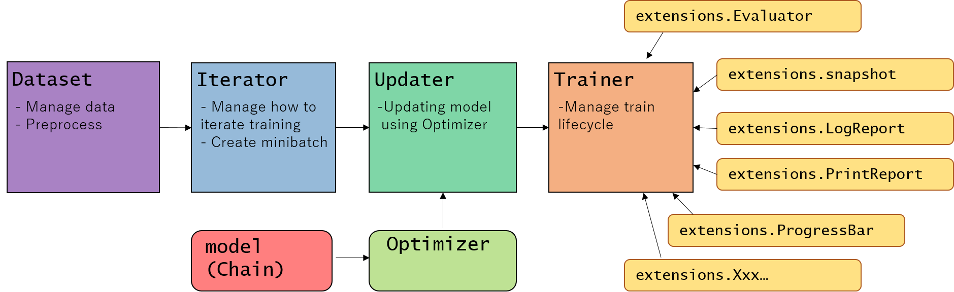
Writing organized, reusable, clean training code using Trainer moduleより
from chainer import iterators, training, optimizers, serializers
from chainer.datasets import TupleDataset
from chainer.training import extensions


# -1 indicates to use CPU,
# positive value indicates GPU device id.
# device = -1  # If you use CPU.
device = 0  # If you use GPU. (You need to install chainer & cupy with CUDA/cudnn installed)
batchsize = 16
class_num = 10
out_dir = '.'
if DEBUG:
    epoch = 5  # This value is small. Change to more than 20 for Actual running.
else:
    epoch = 20


def train_main(train_x, train_y, val_x, val_y, model_path='cnn_model.npz'):
    # 1. Setup model
    model = CNNMedium(n_out=class_num)
    classifier_model = L.Classifier(model)
    if device >= 0:
        chainer.cuda.get_device(device).use()  # Make a specified GPU current
        classifier_model.to_gpu()  # Copy the model to the GPU

    # 2. Setup an optimizer
    optimizer = optimizers.Adam()
    #optimizer = optimizers.MomentumSGD(lr=0.001)
    optimizer.setup(classifier_model)

    # 3. Load the dataset
    #train_data = MNISTTrainImageDataset()
    train_dataset = TupleDataset(train_x, train_y)
    val_dataset = TupleDataset(val_x, val_y)

    # 4. Setup an Iterator
    train_iter = iterators.SerialIterator(train_dataset, batchsize)
    #train_iter = iterators.MultiprocessIterator(train, args.batchsize, n_prefetch=10)
    val_iter = iterators.SerialIterator(val_dataset, batchsize, repeat=False, shuffle=False)

    # 5. Setup an Updater
    updater = training.StandardUpdater(train_iter, optimizer,
                                       device=device)
    # 6. Setup a trainer (and extensions)
    trainer = training.Trainer(updater, (epoch, 'epoch'), out=out_dir)

    # Evaluate the model with the test dataset for each epoch
    trainer.extend(extensions.Evaluator(val_iter, classifier_model, device=device), trigger=(1, 'epoch'))

    trainer.extend(extensions.dump_graph('main/loss'))
    trainer.extend(extensions.snapshot(), trigger=(1, 'epoch'))
    trainer.extend(extensions.LogReport())
    trainer.extend(extensions.PlotReport(
        ['main/loss', 'validation/main/loss'],
        x_key='epoch', file_name='loss.png'))
    trainer.extend(extensions.PlotReport(
        ['main/accuracy', 'validation/main/accuracy'],
        x_key='epoch',
        file_name='accuracy.png'))

    try:
        # Use extension library, chaineripy's PrintReport & ProgressBar
        from chaineripy.extensions import PrintReport, ProgressBar
        trainer.extend(ProgressBar(update_interval=5))
        trainer.extend(PrintReport(
            ['epoch', 'main/loss', 'validation/main/loss',
             'main/accuracy', 'validation/main/accuracy', 'elapsed_time']))

    except:
        print('chaineripy is not installed, run `pip install chaineripy` to show rich UI progressbar')
        # Use chainer's original ProgressBar & PrintReport
        # trainer.extend(extensions.ProgressBar(update_interval=5))
        trainer.extend(extensions.PrintReport(
            ['epoch', 'main/loss', 'validation/main/loss',
             'main/accuracy', 'validation/main/accuracy', 'elapsed_time']))

    # Resume from a snapshot
    # serializers.load_npz(args.resume, trainer)

    # Run the training
    trainer.run()
    # Save the model
    serializers.save_npz('{}/{}'
                         .format(out_dir, model_path), model)
    return model
Trainerを使うことで、学習進捗を示すProgressBarを表示してくれたり、Logを取っておいたり、Loss curveをプロットしたりといった、学習周りのことをサクッと行うことができます。
訓練実行コードは以下のようになります。
import numpy as np
from sklearn.model_selection import train_test_split
seed = 777
model_simple = 'cnn_model_simple.npz'

train_idx, val_idx = train_test_split(np.arange(len(train_x)),
                                      test_size=0.20, random_state=seed)
print('train size', len(train_idx), 'val size', len(val_idx))
train_main(train_imgs[train_idx], train_y[train_idx], train_imgs[val_idx], train_y[val_idx], model_path=model_simple)
- 実行例:
DEBUG=TrueでGPU使用時
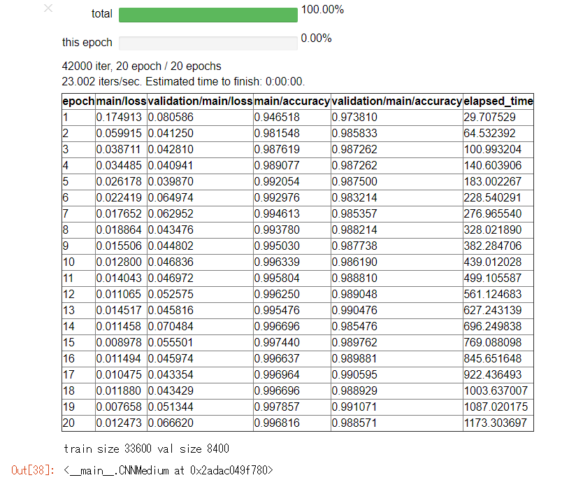
もしchaineripy がインストールされている場合は以下のようなWidget付きのプログレスバーで訓練の進捗を確認することができます。
-
DEBUG=Falseの結果
ラベルの推論を行い、提出用ファイルの作成する
上記で訓練したモデルは保存されているので、これを読み込んで予測を行います。
class_num = 10

def predict_main(model_path='cnn_model.npz'):
    # 1. Setup model
    model = CNNMedium(n_out=class_num)
    classifier_model = L.Classifier(model)
    if device >= 0:
        chainer.cuda.get_device(device).use()  # Make a specified GPU current
        classifier_model.to_gpu()  # Copy the model to the GPU

    # load trained model
    serializers.load_npz(model_path, model)

    # 2. Prepare the dataset --> it's already prepared
    # test_imgs

    # 3. predict the result
    t = model.predict(test_imgs, device=device)
    return t


def create_submission(submission_path, t):
    result_dict = {
        'ImageId': np.arange(1, len(t) + 1),
        'Label': t
    }
    df = pd.DataFrame(result_dict)
    df.to_csv(submission_path,
              index_label=False, index=False)
    print('submission file saved to {}'.format(submission_path))
predict_label = predict_main(model_path=model_simple)
print('predict_label = ', predict_label, predict_label.shape)

create_submission('submission_simple.csv', predict_label)
出力は以下のようになり、提出用ファイル "submission_simple.csv"が作成されました。
predict_label =  [2 0 9 ..., 3 9 2] (28000,)
submission file saved to submission_simple.csv
ファイルを提出: score 0.96400
まずは、第1ステップとしてCNNを実装してMNISTデータセットの学習と推論を行ってみました。
自分の環境では上記のコードで 0.96400 のスコアとなりました。
さて、ここから、さらに精度を上げていく事を考えて行きましょう。
精度改善に何ができるか?
第1ステップでは単純な学習を行いましたが、ここからテストデータに対する精度を上げる(汎化誤差を下げる)ためには、以下のようなテクニックを用いることができます。
- Data augmentation
- モデルアンサンブル
以下ではまず、data augmentationを用いた訓練をChainerでどのように行うかを説明します。
また、Cross validationを行いながらモデルを複数訓練し、その予測結果をアンサンブルして最終結果を予測させてみましょう。
Data augmentation
テストデータに対する精度を上げるためには、訓練データの数・バラエティーが多くなるとよいです。訓練データの数が多ければ、それだけ過学習の影響を減らすことができ、その分テスト精度を上げることができると考えられるからです。
"Data augmentation" は、与えられた訓練データを仮想的に"水増し" するというテクニックです。
実際に例を見てみましょう。
今回の MNIST データセットの分類タスクでは、affine 変換を用いて data augmentation を行うことができます。
- Rotation
- Translation
- Scale
- Shear
from chainer.datasets import TransformDataset
import skimage
import skimage.transform
from skimage.transform import AffineTransform, warp
import numpy as np
def affine_image(img):
#ch, h, w = img.shape
#img = img / 255.
# --- scale ---
min_scale = 0.8
max_scale = 1.2
sx = np.random.uniform(min_scale, max_scale)
sy = np.random.uniform(min_scale, max_scale)
# --- rotation ---
max_rot_angle = 7
rot_angle = np.random.uniform(-max_rot_angle, max_rot_angle) * np.pi / 180.
# --- shear ---
max_shear_angle = 10
shear_angle = np.random.uniform(-max_shear_angle, max_shear_angle) * np.pi / 180.
# --- translation ---
max_translation = 4
tx = np.random.randint(-max_translation, max_translation)
ty = np.random.randint(-max_translation, max_translation)
tform = AffineTransform(scale=(sx, sy), rotation=rot_angle, shear=shear_angle,
translation=(tx, ty))
transformed_image = warp(img[0, :, :], tform.inverse, output_shape=(28, 28))
return transformed_image
transformed_imgs = TransformDataset(train_imgs / 255., affine_image)
print('Affine transformation, image: ', transformed_imgs[0].shape)
# print(train_imgs[0])
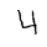
print('Original image')
show_image(train_imgs[3])
print('Transformed image')
show_image(transformed_imgs[3])
show_image(transformed_imgs[3])
結果は以下のようになります。
Affine transformation, image:  (28, 28)
Original image
Transformed image
Affine変換された画像は元の画像と比べてどう見えますか?同じ数字の画像に見えますか(上記の例では4に見えますか)?見えますよね。
このように、画像が少しだけ**回転(Rotation)**されたり、**平行移動(transformed)**されたり、拡大・縮小(scaled) されても、同じラベルの画像に見えます。
このようにして、一つの画像データから何枚もの訓練データを仮想的に作り出すことができます。
[Note] ちなみに、どのようにData augmentationするのが妥当か、というのはタスクによって異なります。今回のMNISTデータセットではAffine 変換を紹介しましたが、自然画像のクラス分類ではその他に左右の反転を行うことなどもできます。
適切なData augmentationはデータの持つ対称性・性質によって異なります。
例えばこちらに自然画像分類のデータセットであるCIFAR-10のData augmentation例があります。
データセットクラスを定義する
上記のようなData augmentationを行いながら学習を行っていくために、Chainerでは自前のデータセットを定義することができます。
以下のように DatasetMixin クラスを継承した自前クラスを定義します。
class MNISTTrainImageDataset(chainer.dataset.DatasetMixin):
    def __init__(self, imgs, labels, train=True, augmentation_rate=1.0,
                 min_scale=0.90, max_scale=1.10, max_rot_angle=4,
                 max_shear_angle=2, max_translation=3):
        self.imgs = imgs.reshape((-1, 1, 28, 28))
        self.labels = labels
        self.train = train

        # affine parameters
        self.augmentation_rate = augmentation_rate
        self.min_scale = min_scale  # 0.85
        self.max_scale = max_scale  # 1.15
        self.max_rot_angle = max_rot_angle  # 5
        self.max_shear_angle = max_shear_angle  # 5
        self.max_translation = max_translation

    def __len__(self):
        """return length of this dataset"""
        return len(self.labels)

    def affine_image(self, img):
        # ch, h, w = img.shape

        # --- scale ---
        sx = np.random.uniform(self.min_scale, self.max_scale)
        sy = np.random.uniform(self.min_scale, self.max_scale)

        # --- rotation ---
        rot_angle = np.random.uniform(-self.max_rot_angle,
                                      self.max_rot_angle) * np.pi / 180.

        # --- shear ---
        shear_angle = np.random.uniform(-self.max_shear_angle,
                                        self.max_shear_angle) * np.pi / 180.

        # --- translation ---
        tx = np.random.randint(-self.max_translation, self.max_translation)
        ty = np.random.randint(-self.max_translation, self.max_translation)

        tform = AffineTransform(scale=(sx, sy), rotation=rot_angle,
                                shear=shear_angle,
                                translation=(tx, ty))
        transformed_image = warp(img[0, :, :], tform.inverse,
                                 output_shape=(28, 28))
        return transformed_image.astype('float32').reshape(1, 28, 28)

    def get_example(self, i):
        """Return i-th data"""
        img = self.imgs[i]
        label = self.labels[i]

        # Data augmentation...
        if self.train:
            if np.random.uniform() < self.augmentation_rate:
                img = self.affine_image(img)

        return img, label
get_example(self, i) の関数で i 番目のデータセット=(i 番目の画像, i 番目のラベル)を返すように実装を行います。
実際に使ってみます。
# 3. Load the dataset
train_data = MNISTTrainImageDataset(train_imgs, train_y)

# train_data[i] is `i`-th dataset, with format (img, label)

# extract 3rd dataset
index = 3
img, label = train_data[index]

show_image(train_data[index][0])
show_image(train_data[index][0])
show_image(train_data[index][0])
同じコード show_image(train_data[index][0]) を何度も実行しただけなのに、異なる画像がプロットされました。
自前のデータセットクラス MNISTTrainImageDataset に対して train_data[index] のようにアクセスを行うと、毎回 get_example(self, i) が呼ばれます。
そのため、毎回 get_example(self, i)内でscale, rotation, shear, translation のパラメータがランダムな値で生成され、Data augmentationが行われたために見える画像が異なるという結果になります。
このデータセットを用いることで、CNN モデルの訓練をData augmentationを行いながら進めることができます。
Training code -- step 2.
Data augmentation のやり方と、それを適用したデータセットクラスの作り方について学んだところで、実際にモデルを MNISTTrainImageDataset を用いて訓練してみましょう。
# -1 indicates to use CPU,
# positive value indicates GPU device id.
device = -1  # If you use CPU.
# device = 0  # If you use GPU. (You need to install chainer & cupy with CUDA/cudnn installed)

batchsize = 16
class_num = 10
out_dir = '.'
if DEBUG:
    epoch = 5  # This value is small. Change to more than 20 for Actual running.
else:
    epoch = 30


def train_main2(train_x, train_y, val_x, val_y, model_path='cnn_model.npz', model_class=CNNMedium):
    # 1. Setup model
    model = model_class(n_out=class_num)
    classifier_model = L.Classifier(model)
    if device >= 0:
        chainer.cuda.get_device(device).use()  # Make a specified GPU current
        classifier_model.to_gpu()  # Copy the model to the GPU

    # 2. Setup an optimizer
    optimizer = optimizers.Adam()
    # optimizer = optimizers.MomentumSGD(lr=0.01)
    optimizer.setup(classifier_model)

    # 3. Load the dataset
    # --- Use custom dataset to train model with data augmentation ---
    train_dataset = MNISTTrainImageDataset(train_x, train_y, augmentation_rate=0.5,
                                           min_scale=0.95, max_scale=1.05, max_rot_angle=7,
                                           max_shear_angle=3, max_translation=2)
    val_dataset = MNISTTrainImageDataset(val_x, val_y, train=False)
    # --- end of modification ---

    # 4. Setup an Iterator
    train_iter = iterators.SerialIterator(train_dataset, batchsize)
    #train_iter = iterators.MultiprocessIterator(train, args.batchsize, n_prefetch=10)
    val_iter = iterators.SerialIterator(val_dataset, batchsize, repeat=False, shuffle=False)

    # 5. Setup an Updater
    updater = training.StandardUpdater(train_iter, optimizer,
                                       device=device)
    # 6. Setup a trainer (and extensions)
    trainer = training.Trainer(updater, (epoch, 'epoch'), out=out_dir)

    # Evaluate the model with the test dataset for each epoch
    trainer.extend(extensions.Evaluator(val_iter, classifier_model, device=device), trigger=(1, 'epoch'))

    # --- Learning rate decay scheduling ---
    def decay_lr(trainer):
        print('decay_lr at epoch {}'.format(trainer.updater.epoch_detail))
        # optimizer.lr *= 0.1  # for MomentumSGD optimizer
        optimizer.alpha *= 0.1
        print('optimizer lr has changed to {}'.format(optimizer.lr))
    trainer.extend(decay_lr,
                   trigger=chainer.training.triggers.ManualScheduleTrigger([10, 20], 'epoch'))
    # --- end of modification ---

    trainer.extend(extensions.dump_graph('main/loss'))
    trainer.extend(extensions.snapshot(), trigger=(1, 'epoch'))
    trainer.extend(extensions.LogReport())
    trainer.extend(extensions.PlotReport(
        ['main/loss', 'validation/main/loss'],
        x_key='epoch', file_name='loss.png'))
    trainer.extend(extensions.PlotReport(
        ['main/accuracy', 'validation/main/accuracy'],
        x_key='epoch',
        file_name='accuracy.png'))

    try:
        # Use extension library, chaineripy's PrintReport & ProgressBar
        from chaineripy.extensions import PrintReport, ProgressBar
        trainer.extend(ProgressBar(update_interval=5))
        trainer.extend(PrintReport(
            ['epoch', 'main/loss', 'validation/main/loss',
             'main/accuracy', 'validation/main/accuracy', 'elapsed_time']))

    except:
        print('chaineripy is not installed, run `pip install chaineripy` to show rich UI progressbar')
        # Use chainer's original ProgressBar & PrintReport
        # trainer.extend(extensions.ProgressBar(update_interval=5))
        trainer.extend(extensions.PrintReport(
            ['epoch', 'main/loss', 'validation/main/loss',
             'main/accuracy', 'validation/main/accuracy', 'elapsed_time']))

    # Resume from a snapshot
    # serializers.load_npz(args.resume, trainer)

    # Run the training
    trainer.run()
    # Save the model
    serializers.save_npz('{}/{}'.format(out_dir, model_path), model)

    return model
step 1 と比べた、上記コードの変更箇所は2つだけです。
1. Dataset を MNISTTrainImageDataset に変更
Data augmentationを行えるように、自作のDatasetクラスを使うように変更しています。
    # 3. Load the dataset
    # --- Use custom dataset to train model with data augmentation ---
    train_dataset = MNISTTrainImageDataset(train_x, train_y, augmentation_rate=0.5,
                                           min_scale=0.95, max_scale=1.05, max_rot_angle=7,
                                           max_shear_angle=3, max_translation=2)
    val_dataset = MNISTTrainImageDataset(val_x, val_y, train=False)
    # --- end of modification ---
2. optimizer に learning rate decay を導入
訓練中に、より細かな精度でロスを最小化できるよう optimizerの learning rate (学習率)を小さくしています。ただし、初めから optimizer の learning rate が小さいと、収束するのに時間がかかってしまいます (*1)。そこで、ここで紹介するように、初めは通常のlearning rateから訓練を初めて、学習途中に徐々にlearning rate を下げていくというテクニックが良く用いられます。
以下のコードは指定した epoch数 (10 epoch目と20 epoch目)に、learning rate を10倍小さな値にする例です。ChainerのTrainerでは、このように 自作 extension をちょこっと追加するだけでこのような学習方法の調整を行うことができます。
    # --- Learning rate decay scheduling ---
    def decay_lr(trainer):
        print('decay_lr at epoch {}'.format(trainer.updater.epoch_detail))
        # optimizer.lr *= 0.1  # for MomentumSGD optimizer
        optimizer.alpha *= 0.1
        print('optimizer lr has changed to {}'.format(optimizer.lr))
    trainer.extend(decay_lr,
                   trigger=chainer.training.triggers.ManualScheduleTrigger([10, 20], 'epoch'))
    # --- end of modification ---
このように、Trainer を用いて訓練コードを書くことにより、学習コードに変更がある場合でも機能を比較的分割して管理することができ、コードの可読性を上げたり、別のプロジェクトで使いまわすこともできます。
モデルをcross validationを用いて訓練する
Cross validation を行うための便利な関数がSklearnから提供されているのでそれをもちいます。
for train_idx, valid_idx in StratifiedKFold(n_splits=N_SPLIT_CV).split(train_imgs, train_y):
というコードを用いることにより、split メソッドの引数である train_imgs, train_y を Train dataと Validation data に分けるためのindex である train_idxと valid_idx を取得することができます。 StratifiedKFold を用いると、train_y に含まれているラベルの情報をみて各ラベルの割合が Train dataとValidation dataで偏らないように自動でバランスを取って Splitを行ってくれます。
以下のコードが実際にcross validationを行いながらモデルを訓練するコードです。
from sklearn.model_selection import KFold, StratifiedKFold

if DEBUG:
    N_SPLIT_CV = 2
else:
    N_SPLIT_CV = 5

cv_step = 0
# for train_idx, valid_idx in StratifiedKFold(n_splits=N_SPLIT_CV, shuffle=True, random_state=7).split(train_imgs, train_y):
for train_idx, valid_idx in StratifiedKFold(n_splits=N_SPLIT_CV).split(train_imgs, train_y):
    print('Training cv={} ...'.format(cv_step))
    train_main2(train_imgs[train_idx], train_y[train_idx],
                train_imgs[val_idx], train_y[val_idx],
                model_path='cnn_model_cv{}.npz'.format(cv_step))
    cv_step += 1
出力サンプル (DEBUG=False)
実際はN_SPLIT_CV の数だけ訓練が繰り返されますが、長いので省略します。
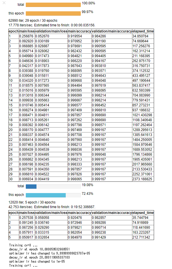
テスト精度(validation/main/accuracy)が 99.9%近くまで出ており、Step 1の時と比べるとものすごく改善されていることがわかります。
また、Step 1の時と比べると、訓練誤差 (main/loss)が収束するまでに少し時間がかかると思います。この原因の一つとしては、Data augmentationを行ったことにより学習中モデルが毎回違う画像を入力しているということが挙げられます。
モデルアンサンブルを行って結果を予測
訓練をCross validationで行ったので、N_SPLIT_CV の数だけモデルが学習されています。
今回は単にこれらのモデルの予測(確率値)の平均値を取って最終結果としてみましょう。
class_num = 10
# device= -1

def predict_proba_main(model_path='cnn_model.npz'):
    # 1. Setup model
    model = CNNMedium(n_out=class_num)
    classifier_model = L.Classifier(model)
    if device >= 0:
        chainer.cuda.get_device(device).use()  # Make a specified GPU current
        classifier_model.to_gpu()  # Copy the model to the GPU

    # load trained model
    serializers.load_npz(model_path, model)

    # 2. Load the dataset
    # test_imgs is already prepared

    # 3. predict the result
    proba = model.predict_proba(test_imgs, device=device)
    return proba


def create_submission(submission_path, t):
    result_dict = {
        'ImageId': np.arange(1, len(t) + 1),
        'Label': t
    }
    df = pd.DataFrame(result_dict)
    df.to_csv(submission_path,
              index_label=False, index=False)
    print('submission file saved to {}'.format(submission_path))
実行します。proba が各モデルの予測確率で、その値をproba_array に格納しています。
proba_list = []
for i in range(N_SPLIT_CV):
    print('predicting {}-th model...'.format(i))
    proba = predict_proba_main(model_path='./cnn_model_cv{}.npz'.format(i))
    proba_list.append(proba)

proba_array = np.array(proba_list)
predicting 0-th model...
predicting 1-th model...
predicting 2-th model...
predicting 3-th model...
predicting 4-th model...
proba_arrayの平均値をproba_ensemble として取ることで最終予測確率を出し、そこから最終予測ラベル predict_ensemble を計算しています。
proba_ensemble = np.mean(proba_array, axis=0)  # Take each model's mean as ensembled prediction.
predict_ensemble = np.argmax(proba_ensemble, axis=1)

# --- Check shape ---
# 0th axis represents each model, 1st axis represents test data index, 2nd axis represents the probability of each label
print('proba_array', proba_array.shape)
# 0th axis represents test data index, 1st axis represents the probability of each label
print('proba_ensemble', proba_ensemble.shape)
# 0th axis represents final label prediction for test data index
print('predict_ensemble', predict_ensemble.shape, predict_ensemble)
proba_array (5, 28000, 10)
proba_ensemble (28000, 10)
predict_ensemble (28000,) [2 0 9 ..., 3 9 2]
最後に予測結果を提出用CSVファイルに書き出して完成です。
create_submission('submission_ensemble.csv', predict_ensemble)
submission file saved to submission_ensemble.csv
提出結果: score 0.99700
これでStep 2もようやく終わりです。Convolutional Neural Networkを用いた学習と、その予測方法について理解できたでしょうか?
今回は、ディープラーニング界隈では広く用いられているテクニックとして、以下を紹介しました。
- data augmentationのやり方、Datasetの作り方
- learning rate のスケジューリングによる、より細かな精度追及
- cross validationの方法
- モデルアンサンブルを行った予測
これらのテクニックを取り入れた結果、自分の環境では、"submission_ensemble.csv"は 0.99700 のスコアを得ることができました。
Appendix: ロスが高いデータの可視化
最後に付録として、これ以上精度を上げるのがどれだけ難しいことなのかについて言及しておきます。
これを考察するために、訓練済みモデルにとって"特に難しいデータ" を見てみたいと思います。
以下のコードはsoftmax cross entropy ロスをそれぞれの訓練データに対して計算し、そのロスが大きいものから順に可視化するコードです。
from chainer import cuda

def calc_loss_and_prob(model_path='cnn_model.npz'):
    # 1. Setup model
    model = CNNMedium(n_out=class_num)
    classifier_model = L.Classifier(model)
    if device >= 0:
        chainer.cuda.get_device(device).use()  # Make a specified GPU current
        classifier_model.to_gpu()  # Copy the model to the GPU

    # load trained model
    serializers.load_npz(model_path, model)

    # 2. Load the dataset
    # test_imgs is already prepared

    # 3. predict the result
    if device >= 0:
        h = model(cuda.to_gpu(train_imgs))
        loss = F.softmax_cross_entropy(h, cuda.to_gpu(train_y), reduce='no')
        return cuda.to_cpu(loss.data), cuda.to_cpu(h.data)
    else:
        h = model(train_imgs)
        loss = F.softmax_cross_entropy(h, train_y)
        return loss.data, h.data
各モデル毎に、ロスと予測値を両方計算し、結果を格納します。
loss_list = []
prob_list = []
for i in range(N_SPLIT_CV):
    print('calc loss for {}-th model...'.format(i))
    loss, prob = calc_loss_and_prob(model_path='./cnn_model_cv{}.npz'.format(i))
    loss_list.append(loss)
    prob_list.append(prob)

loss_array = np.array(loss_list)
prob_array = np.array(prob_list)
calc loss for 0-th model...
calc loss for 1-th model...
calc loss for 2-th model...
calc loss for 3-th model...
calc loss for 4-th model...
各モデルの平均値を取ります。loss_ensemble がLossの値の平均値です。これが高いものがモデルが予測を当てるのが"難しいデータ"だと考えられます。
loss_ensemble = np.mean(loss_array, axis=0)  # Take each model's mean loss.
predict_ensemble = np.mean(prob_array, axis=0)  # Take each model's mean as ensembled prediction.

# --- Check shape ---
# 0th axis represents each model, 1st axis represents test data index, 2nd axis represents the probability of each label
print('loss_array', loss_array.shape)
# 0th axis represents test data index, 1st axis represents the probability of each label
print('loss_ensemble', loss_ensemble.shape)
loss_array (5, 42000)
loss_ensemble (42000,)
ロスの値が大きいもの、小さいもののIndexを見てみます。
loss_index = np.argsort(loss_ensemble)
print('BEST100:  ', loss_index[:30], loss_ensemble[loss_index[:30]])
print('WORST100: ', loss_index[::-1][:100], loss_ensemble[loss_index[::-1][:100]])
BEST100:   [20999 26868 12769 12768 12767 26871 12765 12771 26872 26876 12761 12760
 26877 12758 12757 26874 26865 12773 26864 12789 26843 26846 26849 26852
 26853 26854 26855 26857 12780 12779] [ 0.  0.  0.  0.  0.  0.  0.  0.  0.  0.  0.  0.  0.  0.  0.  0.  0.  0.
  0.  0.  0.  0.  0.  0.  0.  0.  0.  0.  0.  0.]
WORST100:  [16301 37013 36018 24477 15065 25946 36984 14434 21021 12520 23299 35063
 29524  4226 18283 25172 29296 36569 29436  3997 26182   125 36916 25073
 22089 25468 36755 18502 13044 30119  7369 25069 25708 25074 18534 14032
 41691 28560 25619 23135 30275 12706 15219  2381  4967 18316 29496 27489
 12170 34274  2316 18319 12560  7389 14101 17016  8780 23604 23036  5885
 10941  5747  7764 24109 22368 27977  7242  2453 24153 10644 15281 29033
 13477 20172 39331 14121  7505  4169 11406  5124  8566 24230  5659 27335
  6781  5294 15121 13920 24891  7725 26661 30317 28439 23538   897 40257
 30548  4047 18909 19234] [ 8.8119154   5.83190393  5.60041142  4.66397429  2.71987653  2.61653018
  2.50050402  2.48973417  2.12618208  2.10292292  2.08970189  2.0757103
  2.05407429  2.04782724  2.04571033  2.04538107  1.97121549  1.95769727
  1.86957228  1.86723292  1.84788036  1.78277075  1.73426318  1.62813115
  1.60833585  1.59187937  1.57165217  1.51381588  1.50113785  1.4952234
  1.47336733  1.46531606  1.42238045  1.42168951  1.4215219   1.41944909
  1.41319525  1.40870917  1.39675617  1.3652854   1.35680568  1.35350919
  1.34562886  1.31280124  1.22915041  1.22818351  1.2166487   1.21610427
  1.19632399  1.189466    1.17719662  1.14934373  1.14559543  1.11949205
  1.10238314  1.06671739  1.04187071  1.03164542  1.02937222  1.02469218
  1.00059259  0.97318995  0.97223741  0.96988469  0.9641673   0.95173872
  0.94543922  0.93992651  0.93631601  0.9353205   0.92623645  0.92149317
  0.91036212  0.89939797  0.88565809  0.8600651   0.85796469  0.84637845
  0.83733004  0.83040464  0.82955885  0.82606184  0.82579976  0.82267743
  0.8154639   0.81347334  0.80267888  0.80201232  0.79891717  0.79082859
  0.7765857   0.77487582  0.74786758  0.74699199  0.74170196  0.74108636
  0.72523451  0.72086298  0.7155484   0.71360904]
Indexを見てもよくわからないので、可視化してみましょう
def show_images(imgs):
    num_imgs = len(imgs)
    fig, axs = plt.subplots(nrows=1, ncols=num_imgs)
    # plt.figure(figsize=(1.5, 1.5))
    plt.axis('off')
    #if img.ndim == 3:
    #    img = img[0, :, :]
    print('imgs shape', imgs.shape)
    for i in range(num_imgs):
        axs[i].imshow(imgs[i, 0, :, :], cmap=plt.cm.binary)
        axs[i].axis('off')
    plt.show()
worst_index = loss_index[::-1][:10]
print('label ', train_y[worst_index])
print('predict ', np.argmax(predict_ensemble, axis=1)[worst_index])
show_images(train_imgs[worst_index])

# for i in loss_index[::-1][:10]:
#    print('label ', train_y[i])
#    show_images(train_imgs[])
結果は以下のようになりました。
label  [4 4 3 3 9 7 8 4 1 9]
predict  [7 9 9 5 4 1 8 9 1 9]
imgs shape (10, 1, 28, 28)
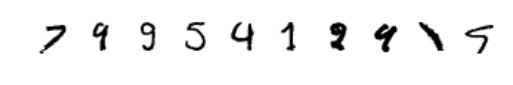
結果を見て、どう思いましたか?
一番左の画像は私には 7 に見えます、そしてCNNモデルも 7 であると予測しています。しかしこの正解ラベルは 4 です。多分、ラベリングの作業にミスがあったのではないかと思います。
このように、データセットには混乱するようなデータもいくつか含まれており、機械学習で精度100% を達成するのはほぼ不可能でしょう。