前回の記事:
TensorFlowの高レベルAPIの使用方法:tf.layersの使い方と重みなどの取り出し方
https://qiita.com/cometscome_phys/items/95ed1b89acc7829950dd
に引き続き、TensorFlowの高レベルAPIを用いてみる。
今回は、Batch Normalization (バッチ正規化)である。
学習用のインプットデータをランダムにピックアップしたものをバッチと呼ぶが、これは、ランダムに何度もピックアップすることで、過学習を避ける仕組みである。
Batch Normalizationとは、ニューラルネットの途中で、バッチの平均を0分散を1に処理:
$$
y \leftarrow \gamma (y-\mu)/\sqrt{\sigma^2+\epsilon} + \beta
$$
する方法である。ここで、$\gamma$と$\beta$は学習される。$\epsilon$はゼロ割を避けるための小さな正の数である。また、トレーニング時には$\mu$はバッチの平均、$\sigma$はバッチの分散が入る。テスト時には$\mu$と$\sigma$は移動平均と移動分散を入れることになる。
これを用いると、収束の高速化などが期待される。
原論文は
Sergey Ioffe, Christian Szegedy,
"Batch Normalization: Accelerating Deep Network Training by Reducing Internal Covariate Shift"
https://arxiv.org/abs/1502.03167
にある。
日本語の解説などは
https://qiita.com/t-tkd3a/items/14950dbf55f7a3095600
等がわかりやすい。
TensorFlowでは、高レベルAPIにBatch Normalizationが実装されているので、そちらを使ってみる。
追記 もう少しスマートなやり方がわかったので追記している。
バージョン
TensorFlow: 1.4.1
Python: 3.6.4
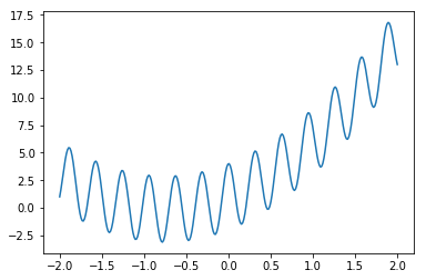
再現すべき関数
前回の記事と同じ関数である。
import tensorflow as tf
import numpy as np
import matplotlib.pyplot as plt
%matplotlib inline

n = 10
x0 = np.linspace(-2.0, 2.0, n)
a0 = 3.0
a1 = 2.0
b0 = 1.0
y0 = np.zeros((n,1))
y0[:,0] = a0*x0+a1*x0**2 + b0 + 3*np.cos(20*x0)

nm = 300
xmany = np.linspace(-2.0, 2.0, nm)
ymany = np.zeros((nm,1))
ymany[:,0] = a0*xmany+a1*xmany**2 + b0 + 3*np.cos(20*xmany)

plt.plot(xmany,ymany )
plt.show()
plt.savefig("graph_many.png")
ランダムバッチ:バッチ正規化なし
まずはじめに、バッチ正規化なしの場合を考える。トレーニングの際にランダムにバッチを選んでくることで、特定のバッチに過学習されることを防ぐことができる。
グラフの構築
前回の記事と同じである。
def build_graph_layers_class(d_input,d_middle,d_type):
    x = tf.placeholder(shape=[None,d_input],dtype=d_type)
    yout = tf.placeholder(shape=[None,1],dtype=d_type)
    hidden1 = tf.layers.Dense(units=d_middle,activation=tf.nn.relu)
    x1 = hidden1(x)
    outlayer = tf.layers.Dense(units=1,activation=None)
    y = outlayer(x1)

    diff = tf.subtract(y,yout)
    loss = tf.nn.l2_loss(diff)
    minimize = tf.train.AdamOptimizer().minimize(loss)
    return x,y,yout,diff,loss,minimize,hidden1,outlayer
TensorFlowのtf.layersを使うことでシンプルに表現できる。
また、レイヤーに関するインスタンスを定義することで、重みなどが取り出しやすくなっている。
グラフの実行
前回の記事とよく似ている。なお、インプットとしては5次までの多項式を使い、隠れ層は一層である。ユニットの数は10個である。
tf.reset_default_graph()

k = 6
phi = make_phi(x0,n,k)
phimany = make_phi(xmany,nm,k)
d_type = tf.float32
d_input = k
d_middle = 10
x,y,yout,diff,loss,minimize,hidden1,outlayer= build_graph_layers_class(d_input,d_middle,d_type)
gpunum = 0
config = tf.ConfigProto(
    gpu_options=tf.GPUOptions(
    visible_device_list=str(gpunum), # specify GPU number
    allow_growth=True
        )
    )

batchsize = 20
with tf.Session(config=config) as sess:
    tf.global_variables_initializer().run()
    nt = 2000
    vec_loss = []
    vec_loss_many = []
    for i in range(nt):
        A = np.arange(nm)
        np.random.shuffle(A)
        data_out = np.array([ymany[A[j]] for j in range(batchsize)])
        data_inp = np.array([phimany[A[j],:] for j in range(batchsize)])

        sess.run(minimize, feed_dict={x: data_inp,yout: data_out})

        losstrain = sess.run(loss, feed_dict={x: data_inp,yout: data_out})/batchsize
        losstrain_many = sess.run(loss, feed_dict={x: phimany,yout: ymany})/nm
        vec_loss.append(losstrain)
        vec_loss_many.append(losstrain_many)
        if i % 100 is 0:
            print("i",i,"loss",losstrain_many)


    ye = sess.run(y, feed_dict={x: phi})
    yemany = sess.run(y, feed_dict={x: phimany})
    W = sess.run(hidden1.weights)
    print(W)
    a = sess.run(outlayer.weights)
    print(a)


plt.plot(xmany,ymany)
plt.plot(xmany,yemany,'v')

plt.show()
plt.savefig("graph_2_layers_class.png")

plt.plot(vec_loss,label = "Training data")
plt.plot(vec_loss_many,label = "Test data")
plt.legend()
plt.show()
plt.savefig("loss.png")
GPUを使うことを想定してSessionに使うGPUの番号を入れるようにconfigを設定している。
毎回20個のデータ点を取ってきており、それを用いて学習をしている。
lossについては、トレーニングデータ20個の場合と、テストデータ300点の場合をそれぞれ計算している。
最後に、得られたフィッティングの結果をプロットし、lossの変化もプロットした。
フィッティングの結果は、
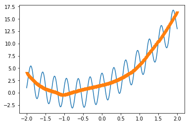
である。cosの振動に騙されずに真ん中を通るようにフィッティングされていることがわかる。多分、もう少しパラメータをチューニングすればいいものが得られるはずである。
lossの変化は
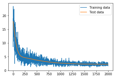
となっている。もともとそんなに複雑な関数ではないからか、あっさりと落ちている。
ランダムバッチ:バッチ正規化あり
TensorFlowのバージョン1.4から、高レベルAPIにクラスが実装され、とても便利になった。
しかし、英語日本語共にweb文献がほとんどなかったため、実装に苦労した。
Batch Normalizationに関しては、
- tf.nn.batch_normalization
- tf.layers.batch_normalization
を使う方法が多い。今回は、クラス
- tf.layers.BatchNormalization
を使った方法を実装する。こちらを使うと、インスタンスから移動平均、移動分散などの量を簡単に取ることができる。
グラフの構築
def build_graph_layers_class_BN(d_input,d_middle,d_type):
    x = tf.placeholder(shape=[None,d_input],dtype=d_type)
    yout = tf.placeholder(shape=[None,1],dtype=d_type)
    hidden1 = tf.layers.Dense(units=d_middle,activation=tf.nn.relu)
    x1 = hidden1(x)
    BN = tf.layers.BatchNormalization()
    x_BN = BN(x1,training=True)
    outlayer = tf.layers.Dense(units=1,activation=None)
    y = outlayer(x_BN)

    diff = tf.subtract(y,yout)
    loss = tf.nn.l2_loss(diff)
    minimize = tf.train.AdamOptimizer().minimize(loss)
    extra_update_ops = tf.get_collection(tf.GraphKeys.UPDATE_OPS)

    return x,y,yout,diff,loss,minimize,hidden1,outlayer,BN,extra_update_ops
ここで、ポイントは、大文字から始まるBatchNormalizationを使っていることと、extra_update_opsを定義していることである。それ以外は先ほどのグラフと変わらない。
なお、extra_update_opsを実行しない限り、移動平均、移動分散(moving_mean,moving_variance)が学習の過程で更新されず、学習が終わった時のテストの際に使うことができない。これに気がつくまでに時間がかかってしまった。
こちらの
https://stackoverflow.com/questions/43234667/tf-layers-batch-normalization-large-test-error
26番の回答を参考にした。
なお、BN(x1,training=True)をBN(x1)とすると移動平均と移動分散が更新されない。原因はよくわからない。
グラフの実行
グラフの実行は
tf.reset_default_graph()

k = 6
phi = make_phi(x0,n,k)
phimany = make_phi(xmany,nm,k)
d_type = tf.float32
d_input = k
d_middle = 10
x,y,yout,diff,loss,minimize,hidden1,outlayer,BN,extra_update_ops= build_graph_layers_class_BN(d_input,d_middle,d_type)
gpunum = 0
config = tf.ConfigProto(
    gpu_options=tf.GPUOptions(
    visible_device_list=str(gpunum), # specify GPU number
    allow_growth=True
        )
    )

batchsize = 20
with tf.Session(config=config) as sess:
    tf.global_variables_initializer().run()
    nt = 2000
    vec_loss_BN = []
    vec_loss_many_BN = []
    for i in range(nt):
        A = np.arange(nm)
        np.random.shuffle(A)
        data_out = np.array([ymany[A[j]] for j in range(batchsize)])
        data_inp = np.array([phimany[A[j],:] for j in range(batchsize)])

        sess.run([minimize,extra_update_ops], feed_dict={x: data_inp,yout: data_out})

        losstrain = sess.run(loss, feed_dict={x: data_inp,yout: data_out})/batchsize
        losstrain_many = sess.run(loss, feed_dict={x: phimany,yout: ymany})/nm
        vec_loss_BN.append(losstrain)
        vec_loss_many_BN.append(losstrain_many)
        if i % 100 is 0:
            print("i",i,"loss",losstrain_many)


    ye = sess.run(y, feed_dict={x: phi})
    yemany = sess.run(y, feed_dict={x: phimany})
    W = sess.run(hidden1.weights)
    print(W)
    a = sess.run(outlayer.weights)
    print(a)
    BN_w = sess.run(BN.weights)
    print(BN_w)
でできる。ここで、sess.runのところでminimize,extra_update_opsの二つを呼んでいることに注意。
最後には、学習して得られた結果を出力している。BN_wに関しては、$\gamma$, $\beta$, 移動平均、移動分散、の順で格納されているようである。
plt.plot(xmany,ymany)
plt.plot(xmany,yemany,'v')

plt.show()
plt.savefig("graph_2_layers_class_BN.png")

plt.plot(vec_loss_BN,label = "Training data")
plt.plot(vec_loss_many_BN,label = "Test data")
plt.legend()
plt.show()
plt.savefig("loss_BN.png")

plt.plot(vec_loss_many,label = "Test data without BN")
plt.plot(vec_loss_many_BN,label = "Test data with BN")
plt.legend()
plt.show()
plt.savefig("loss_test.png")

plt.yscale("log")
plt.plot(vec_loss_many,label = "Test data without BN")
plt.plot(vec_loss_many_BN,label = "Test data with BN")
plt.legend()
plt.show()
plt.savefig("loss_testlog.png")
先ほどの場合と比較するためにグラフを出してみた。
まず、フィッティングした関数は
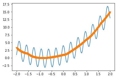
となり、いい感じになっている。
lossは
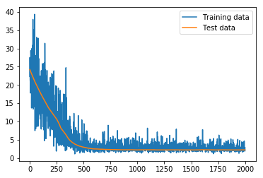
となっている。
テストデータに対して、バッチ正規化ありとなしでどう違うか見てみると、
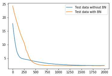
となり、落ち方がバッチ正規化の方が速い。
また、logで見てみると、
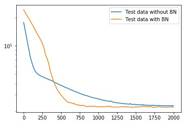
となり、素早く落ちているのがわかりやすい。
追記
tf.layersのソースコード
https://github.com/tensorflow/tensorflow/blob/r1.4/tensorflow/python/layers/normalization.py
を眺めてみたところ、やはりtrainingという値がFalseだと移動平均と移動分散は更新されていないようだ。これがFalseだと、保持している移動平均と移動分散を用いてnn.batch_normalizationを呼んでいる。つまり、これはテスト時の動きになっている。
したがって、トレーニングの時にはTrueにする必要がある。
以上をふまえてグラフを構築すると
def build_graph_layers_class_BN(d_input,d_middle,d_type):
    is_training = tf.placeholder_with_default(False,shape=[])
    x = tf.placeholder(shape=[None,d_input],dtype=d_type)
    yout = tf.placeholder(shape=[None,1],dtype=d_type)
    hidden1 = tf.layers.Dense(units=d_middle,activation=tf.nn.relu)
    x1 = hidden1(x)
    BN = tf.layers.BatchNormalization()
    x_BN = tf.cond(is_training,lambda: BN(x1,training=True),lambda: BN(x1,training=False))
    outlayer = tf.layers.Dense(units=1,activation=None)
    y = outlayer(x_BN)

    diff = tf.subtract(y,yout)
    loss = tf.nn.l2_loss(diff)
    update_ops = tf.get_collection(tf.GraphKeys.UPDATE_OPS)
    with tf.control_dependencies(update_ops):
        minimize = tf.train.AdamOptimizer().minimize(loss)

    return x,y,yout,diff,loss,minimize,hidden1,outlayer,BN,is_training
となる。ここで、わざわざupdate_upsを呼ぶのは面倒なので、minimizeを実行するときは必ずupdate_opsを呼んでねという形になるようにwithを用いた。
また、tf.condはTensorFlowでのIf文である。is_trainingという値のデフォルトをFalseにしておいて、トレーニングする時のみis_training: Trueとできるように変更した。
その時のグラフの実行は
tf.reset_default_graph()

k = 6
phi = make_phi(x0,n,k)
phimany = make_phi(xmany,nm,k)
d_type = tf.float32
d_input = k
d_middle = 10
x,y,yout,diff,loss,minimize,hidden1,outlayer,BN,is_training= build_graph_layers_class_BN(d_input,d_middle,d_type)
gpunum = 0
config = tf.ConfigProto(
    gpu_options=tf.GPUOptions(
    visible_device_list=str(gpunum), # specify GPU number
    allow_growth=True
        )
    )

batchsize = 20
with tf.Session(config=config) as sess:
    tf.global_variables_initializer().run()
    nt = 2000
    vec_loss_BN = []
    vec_loss_many_BN = []
    for i in range(nt):
        A = np.arange(nm)
        np.random.shuffle(A)
        data_out = np.array([ymany[A[j]] for j in range(batchsize)])
        data_inp = np.array([phimany[A[j],:] for j in range(batchsize)])

        sess.run(minimize, feed_dict={x: data_inp,yout: data_out,is_training:True})

        losstrain = sess.run(loss, feed_dict={x: data_inp,yout: data_out})/batchsize
        losstrain_many = sess.run(loss, feed_dict={x: phimany,yout: ymany})/nm
        vec_loss_BN.append(losstrain)
        vec_loss_many_BN.append(losstrain_many)

        if i % 100 is 0:
            print("i",i,"loss",losstrain_many)


    ye = sess.run(y, feed_dict={x: phi})
    yemany = sess.run(y, feed_dict={x: phimany})
    W = sess.run(hidden1.weights)
    print(W)
    a = sess.run(outlayer.weights)
    print(a)
    BN_w = sess.run(BN.weights)
    print(BN_w)
となる。sess.runでminimizeを呼ぶときだけ、feed_dictにis_trainingを指定する形になっている。
まとめ
tf.layersのクラスtf.layers.BatchNormalizationを用いて、バッチ正規化を実装してみた。このやり方だと、重みや移動平均が取り出しやすい。update_opsに注意すること。