これまでJuliaでTensorFlowを使う記事をいくつか書いたが、今回はPython 3を使って、TensorFlow.layersを使ってみる。
これはとても便利らしいが、Web上の文献があまりないため、試行錯誤した。
この記事には三種類の方法を記述してある。tf.layersを使わないやり方、tf.layersを使ったやり方二通り(クラスを使わないやり方と使うやり方)である。
三番目のやり方を使うと、とても簡単に学習後の重みなどを表示できる。
以前の
JuliaでTensorFlow その5: ニューラルネットワークの導入と深層学習
https://qiita.com/cometscome_phys/items/45017aa9741c5fdc7eb9
で扱った問題をPythonに移植し、tf.layersを使っている。
TensorFlowや扱っている問題については、この記事を参照。
TensorFlowそのものについては、
JuliaでTensorFlow その1
https://qiita.com/cometscome_phys/items/358bc4a1feaec1c7fa14
等にも説明してある。
前回の記事で言及した過学習を避けるためのランダムバッチのやり方についてはここでは扱わず、得られた結果をフィッティングすることにのみ注力する。
バージョン
TensorFlow: 1.4.1
Python: 3.6.4
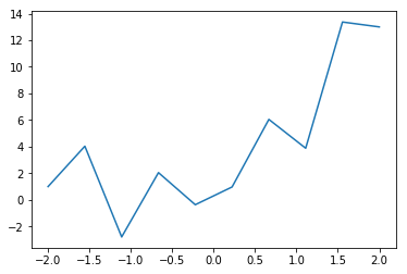
再現すべき関数
import tensorflow as tf
import numpy as np
import matplotlib.pyplot as plt
%matplotlib inline

n = 10
x0 = np.linspace(-2.0, 2.0, n)
a0 = 3.0
a1 = 2.0
b0 = 1.0
y0 = np.zeros((n,1))
y0[:,0] = a0*x0+a1*x0**2 + b0 + 3*np.cos(20*x0)

plt.plot(x0,y0 )
plt.show()
plt.savefig("graph.png")
よくあるやり方
まず、Julia版TensorFlowと似たような形で、グラフを定義してみる。なお、後半にtf.layersを関係上、ベクトルと行列の積が以前のと転置の関係になっていることに注意。また、他の問題に応用しやすいように、あえて定数項$b$を足してある。
グラフの構築
def build_graph(d_input,d_middle,d_type):
    x = tf.placeholder(shape=[None,d_input],dtype=d_type)
    yout = tf.placeholder(shape=[None,1],dtype=d_type)
    a = tf.Variable(tf.zeros([d_middle,1],dtype=d_type),dtype=d_type)
    b = tf.Variable(tf.zeros([1],dtype=d_type),dtype=d_type)

    W = tf.Variable(tf.random_normal([d_input,d_middle],dtype=d_type),dtype = d_type)
    xW = tf.matmul(x,W)
    xWb = tf.add(xW,b)
    x1 = tf.nn.relu(xWb)
    b1 = tf.Variable(tf.zeros([1],dtype=d_type),dtype=d_type)
    x1a = tf.matmul(x1,a)
    y = tf.add(x1a,b1)

    diff = tf.subtract(y,yout)
    loss = tf.nn.l2_loss(diff)
    minimize = tf.train.AdamOptimizer().minimize(loss)
    return x,a,y,yout,diff,loss,minimize,W,b,b1
インプットは多項式であり、隠れ層が何もなければ多項式による線形回帰となる。インプットは
def make_phi(x0,n,k):
    phi = np.array([x0**j for j in range(k)])
    return phi.T
で定義しておく。
3次関数までをインプットにした場合、
グラフの実行
グラフの実行は
tf.reset_default_graph()

k = 4
phi = make_phi(x0,n,k)
d_type = tf.float32
d_input = k
d_middle = 10
x,a,y,yout,diff,loss,minimize,W,b,b1 = build_graph(d_input,d_middle,d_type)

with tf.Session() as sess:
    tf.global_variables_initializer().run()
    nt = 20000
    for i in range(nt):
        sess.run(minimize, feed_dict={x: phi,yout: y0})
        if i %1000 is 0:
            losstrain = sess.run(loss, feed_dict={x: phi,yout: y0})
            print(i,losstrain)

    ye = sess.run(y, feed_dict={x: phi,yout: y0})
    We =  sess.run(W)
    print("W = ",We)
    be =  sess.run(b)
    print("b = ",be)
    ae =  sess.run(a)
    print("a = ",ae)
    be1 =  sess.run(b1)
    print("b1 = ",be1)

plt.plot(x0,y0 )
plt.plot(x0,ye,'o')
plt.show()
plt.savefig("graph_2.png")
で、
得られる図は
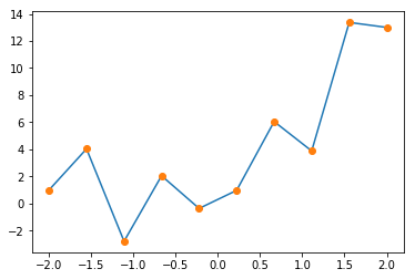
である。
この時の重みの値は
W =  [[-3.823791   -0.2909244   3.7424092   2.3284013  -2.3505242  -3.0136676
  -3.0102415  -1.5948302   2.39074     2.0128825 ]
 [-0.8010104   2.2826529   0.60734206 -0.9295354   1.2737343  -0.1454193
  -0.57141984  1.2848969   0.76956147 -2.4907932 ]
 [ 4.176712   -0.74359405  0.87909096 -0.7212285  -0.55974334  3.5484672
   3.5768263   4.5544047  -0.63729817 -0.8496621 ]
 [-0.49180672 -1.1368665   1.5925783   1.8705708  -1.4488153  -3.7382941
  -3.66106    -2.427403    0.626671    2.7832117 ]]
b =  [0.23165765]
a =  [[ 2.6452117]
 [10.681901 ]
 [-2.7177508]
 [ 1.4725704]
 [-3.234591 ]
 [-3.8175602]
 [-2.3326735]
 [ 6.1676993]
 [ 0.7261172]
 [ 1.7289842]]
b1 =  [-0.31392455]
と出力される。
tf.layersなやり方:通常版
次に、tf.layersを使ったやり方を見てみよう。
これを使うとニューラルネットをとても簡単に書くことができる。
グラフの構築
グラフの構築は
def build_graph_layers(d_input,d_middle,d_type):
    x = tf.placeholder(shape=[None,d_input],dtype=d_type)
    yout = tf.placeholder(shape=[None,1],dtype=d_type)
    x1 = tf.layers.dense(inputs=x,units=d_middle,activation=tf.nn.relu)
    y = tf.layers.dense(inputs=x1,units=1,activation=None)

    diff = tf.subtract(y,yout)
    loss = tf.nn.l2_loss(diff)
    minimize = tf.train.AdamOptimizer().minimize(loss)
    return x,y,yout,diff,loss,minimize
となり、Variablesの形状などを指定する必要がない。ただLayerを重ねていけばよい。
グラフの実行
グラフの実行は、全く変わらず、
tf.reset_default_graph()

k = 4
phi = make_phi(x0,n,k)
d_type = tf.float32
d_input = k
d_middle = 10
x,y,yout,diff,loss,minimize= build_graph_layers(d_input,d_middle,d_type)

with tf.Session() as sess:
    tf.global_variables_initializer().run()
    nt = 20000
    for i in range(nt):
        sess.run(minimize, feed_dict={x: phi,yout: y0})
        if i %1000 is 0:
            losstrain = sess.run(loss, feed_dict={x: phi,yout: y0})
            print(i,losstrain)

    ye = sess.run(y, feed_dict={x: phi,yout: y0})


plt.plot(x0,y0 )
plt.plot(x0,ye,'v')
plt.show()
plt.savefig("graph_2_layers.png")
で良い。
結果は

となる。
tf.layersなやり方:Class版
tf.layersはとても簡単にニューラルネットを構築できるが、途中途中の$W$やら$b$はどうやって取り出すのだろうか。
上のやり方でも
https://stackoverflow.com/questions/45372291/how-to-get-weights-in-tf-layers-dense
をみる限りやり方はあるのだが、ここで述べるクラスとインスタンスを使った方法が非常に簡単だったので、それを述べる。
グラフの構築
グラフの構築は
def build_graph_layers_class(d_input,d_middle,d_type):
    x = tf.placeholder(shape=[None,d_input],dtype=d_type)
    yout = tf.placeholder(shape=[None,1],dtype=d_type)
    hidden1 = tf.layers.Dense(units=d_middle,activation=tf.nn.relu)
    x1 = hidden1(inputs=x)
    outlayer = tf.layers.Dense(units=1,activation=None)
    y = outlayer(inputs=x1)

    diff = tf.subtract(y,yout)
    loss = tf.nn.l2_loss(diff)
    minimize = tf.train.AdamOptimizer().minimize(loss)
    return x,y,yout,diff,loss,minimize,hidden1,outlayer
となる。ここで、新しくhidden1とoutlayerというインスタンスを定義している。そして、tf.layers.Denseを使っており、tf.layers.denseでないことに注意。大文字を使うとインスタンスを定義できる。インスタンスを定義すると、重みなどを簡単に取り出すことができる。
グラフの実行
tf.reset_default_graph()

k = 4
phi = make_phi(x0,n,k)
d_type = tf.float32
d_input = k
d_middle = 10
x,y,yout,diff,loss,minimize,hidden1,outlayer= build_graph_layers_class(d_input,d_middle,d_type)

with tf.Session() as sess:
    tf.global_variables_initializer().run()
    nt = 20000
    for i in range(nt):
        sess.run(minimize, feed_dict={x: phi,yout: y0})
        if i %1000 is 0:
            losstrain = sess.run(loss, feed_dict={x: phi,yout: y0})
            print(i,losstrain)

    ye = sess.run(y, feed_dict={x: phi,yout: y0})
    W = sess.run(hidden1.weights)
    print(W)
    a = sess.run(outlayer.weights)
    print(a)


plt.plot(x0,y0 )
plt.plot(x0,ye,'v')
plt.show()
plt.savefig("graph_2_layers_class.png")
基本的に前の二つと同じである。違うのは、sess.runでhidden1とoutlayerからweightsを取り出しているところだけである。
結果は、
[array([[-1.1092665 ,  0.21458124,  0.81234753,  1.313479  , -2.0177524 ,
         0.9229844 ,  0.12684834, -0.4461583 , -1.1588777 ,  2.205203  ],
       [-1.8913395 , -0.2215695 , -0.4877039 , -0.8681269 ,  1.6817354 ,
         0.45479074,  0.98038745, -0.29166391,  2.155542  , -1.8705736 ],
       [ 0.03240798, -1.8133143 , -1.532448  ,  0.61596954,  2.7005427 ,
         0.29577184,  1.3201405 , -0.49920312,  3.1197407 , -0.93365496],
       [-2.350614  , -2.4765186 , -3.1657784 , -1.7202485 , -0.9948349 ,
         0.86931664, -0.14774853,  0.3263613 , -1.2519372 ,  1.7189637 ]],
      dtype=float32), array([-0.46591416,  0.6278687 ,  0.2945194 ,  1.2502502 , -1.8204086 ,
        0.65430856, -0.2478724 ,  0.        , -1.1778233 ,  2.0317798 ],
      dtype=float32)]
[array([[-4.48896   ],
       [-3.2777092 ],
       [-2.5224724 ],
       [ 5.38478   ],
       [ 3.7768526 ],
       [ 0.9577403 ],
       [ 1.6757046 ],
       [-0.38825402],
       [ 2.1190248 ],
       [-2.40766   ]], dtype=float32), array([-0.1657266], dtype=float32)]
となり、配列の形で得られていることがわかる。
グラフは
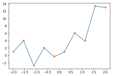
となる。