はじめに
今回私は最近はやりのchatGPTに興味を持ち、深層学習について学んでみたいと思い立ちました!
深層学習といえばPythonということなので、最終的にはPythonを使って深層学習ができるとこまでコツコツと学習していくことにしました。
ただ、勉強するだけではなく少しでもアウトプットをしようということで、備忘録として学習した内容をまとめていこうと思います。
この記事が少しでも誰かの糧になることを願っております!
※投稿主の環境はWindowsなのでMacの方は多少違う部分が出てくると思いますが、ご了承ください。
最初の記事:Python初心者の備忘録 #01
前の記事:Python初心者の備忘録 #25 ~深層学習超入門編01~
次の記事:Python初心者の備忘録 #27 ~深層学習超入門編03~
今回はMLP、誤差逆伝播についてまとめております。
■学習に使用している資料
Udemy:①米国AI開発者がやさしく教える深層学習超入門第一弾【Pythonで実践】
■MLP(Multi-Layer Perceptron:多層パーセプトロン)
▶MLPとは
- MLPの説明に入る前にまずはロジスティック回帰をニューラルネットワーク(NN)で表示した場合の図を紹介する
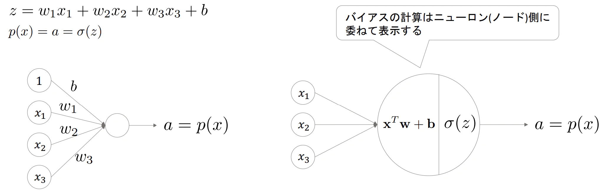
- NNでは通常上図のようなニューロンが並列にいくつも存在する
それがいわゆる多層パーセプトロン(MLP)と呼ばれるもので下図のようになる
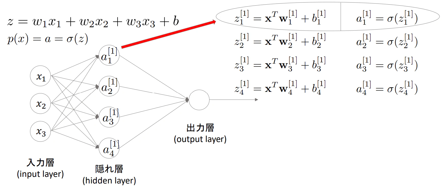
※一般的にMPLでは入力層は総数にカウントせず、次の層からカウントする。(なので、図は2層のMLPとなる)
※※$a_1^{[1]}$の$[1]$は何層目かを表している。
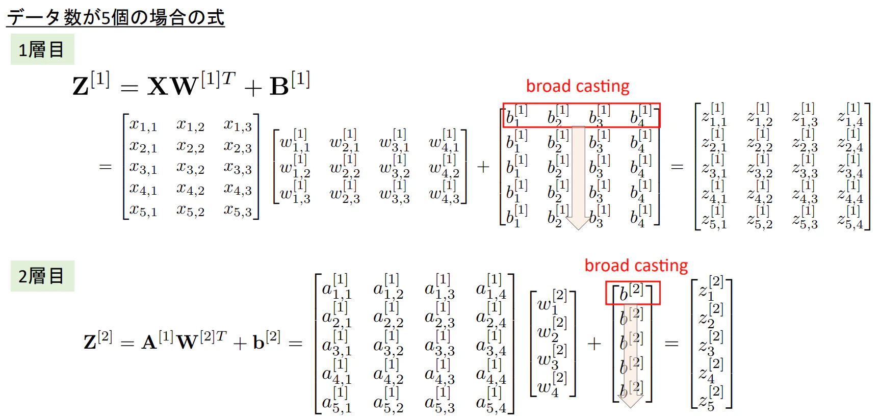
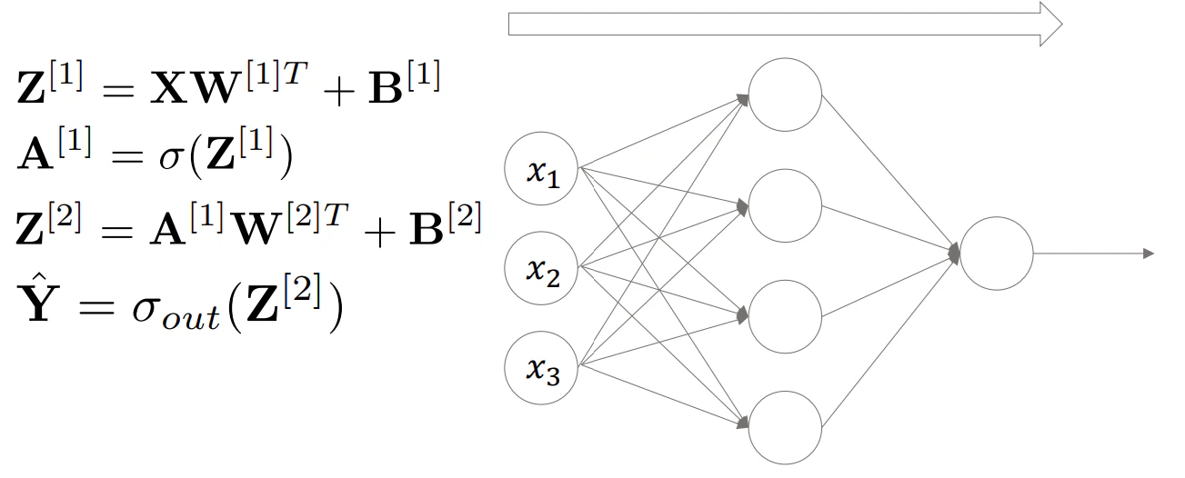
- NNの図を行列としてあらわした場合、下図のようになる
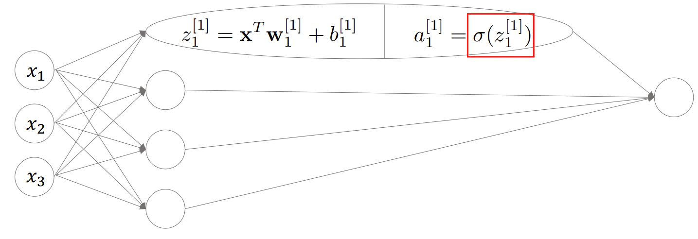
▶活性化関数(activation function)
- 図でも出てきていた$\sigma(z)$のことを活性化関数と呼ぶ
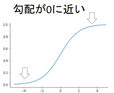
- 基本的最後の出力には活性化関数にシグモイド関数やソフトマックス関数を使用するのだが、それ以外の隠れ層ではまた違ったものを使用する
※シグモイド関数は勾配が0に近くなってしまう点があり、指数関数により計算コストが高いため、隠れ層の活性化関数としては適さない
ではどのような活性化関数を選択すればいいのか?
- 非線形関数を選択する
※活性化関数が線形だと、層を重ねても1つの線形返還になってしまうため - 一般的にはReLU関数が使用される
▶ReLU関数(Rectified Linear Unit)
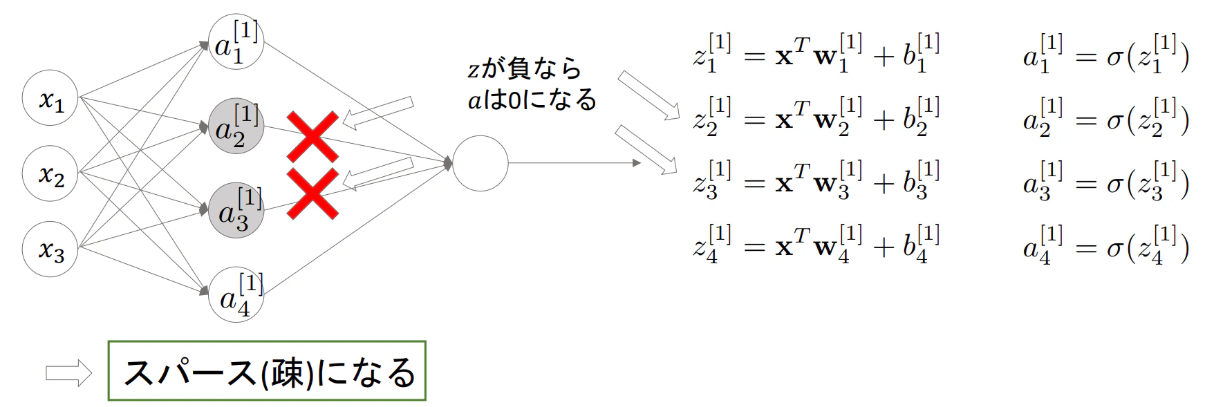
- 一般的に使用される活性化関数で、入力が0以下の場合0を出力し、0以上の場合は入力をそのまま出力する
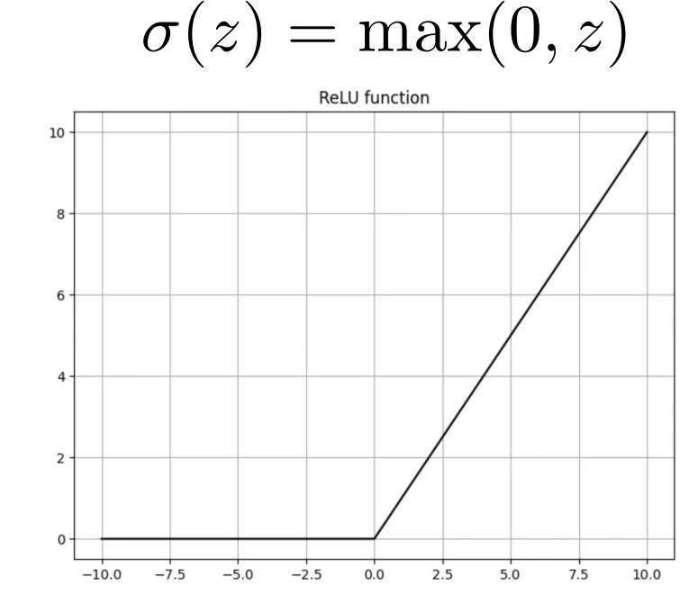
- ReLUを使用することで一部のニューロンのみがアクティブになり、計算効率の向上や過学習の防止を期待できる
- ReLU関数の派生でLeaky ReLUというものもある
- 入力が0未満でも小さな勾配を持つ
※勾配を完全になくさないことで、ある範囲の入力に対して出力が全く変わらない問題を防ぐ
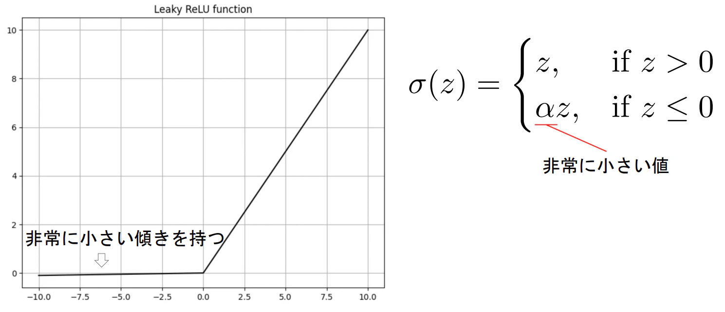
- 入力が0未満でも小さな勾配を持つ
▶出力層の活性化関数
- タスクによって様々
- 2値分類ならシグモイド、多クラス分類ならsoftmax、回帰なら恒等関数
※出力層の活性化関数は恒等関数を使用し、損失関数側で活性化関数を適用することもある(Pytorchではそのような実装になっている)
- 2値分類ならシグモイド、多クラス分類ならsoftmax、回帰なら恒等関数
▶スクラッチでMLPを実装
- 下記条件でMPLを実装する
- 隠れ層のニューロンの数:30
- 隠れ層の活性化関数にはReLUを使用
- モデルの関数を作成し、順伝播で予測した結果を返す
- データはMNISTを使用し、学習用と検証用に分割する
import torch
from sklearn import datasets
import matplotlib.pyplot as plt
from torch.nn import functional as F
from sklearn.model_selection import train_test_split

## データ準備
# 1. データロード
dataset = datasets.load_digits()
images = dataset['images']
target = dataset['target']

# 学習データと検証データ分割
X_train, X_val, y_train, y_val = train_test_split(images, target, test_size=0.2, random_state=42)
print(X_train.shape, y_train.shape)
print(X_val.shape, y_val.shape)

# 前処理
# 2-1.ラベルのone-hot encoing
y_train = F.one_hot(torch.tensor(y_train), num_classes=10)
X_train = torch.tensor(X_train, dtype=torch.float32).reshape(-1, 64)

y_val = F.one_hot(torch.tensor(y_val), num_classes=10)
X_val = torch.tensor(X_val, dtype=torch.float32).reshape(-1, 64)

# 2-2. 画像の標準化
X_train_mean = X_train.mean()
X_train_std = X_train.std()
X_train = (X_train - X_train_mean) / X_train_std
X_val = (X_val - X_train_mean) / X_train_std

# MPL(順伝搬のみ)
m, n = X_train.shape
nh = 30
class_num = 10

# パラメータの初期化
W1 = torch.randn((nh, n), requires_grad=True) # 出力 x 入力
b1 = torch.zeros((1, nh), requires_grad=True) # 1 x nh

W2 = torch.randn((class_num, nh), requires_grad=True) # 出力 x 入力
b2 = torch.zeros((1, class_num), requires_grad=True) # 1 x nh

# 第1層(隠れ層)の計算
def linear(X, W, b):
    return X@W.T + b

# ReLU(隠れ層の活性化関数)
def relu(Z):
    return Z.clamp_min(0.)

# 出力層の活性化関数
def softmax(x):
    # xが大きすぎると,exp(x)がinfになるので,maxを引くようにする(結果は変わらない)
    e_x = torch.exp(x - torch.max(x, dim=-1, keepdim=True)[0])
    return e_x / (torch.sum(e_x, dim=-1, keepdim=True) + 1e-10)

def model(X):
    Z1 = linear(X, W1, b1)
    A1 = relu(Z1)
    Z2 = linear(A1, W2, b2)
    A2 = softmax(Z2)
    return A2

y_train_pred = model(X_train)
y_train_pred
"""
tensor([[1.0000e+00, 1.7962e-41, 2.2879e-22,  ..., 1.1210e-44, 0.0000e+00,
         0.0000e+00],
        [1.0000e+00, 2.4464e-30, 1.0893e-13,  ..., 6.1829e-40, 2.5243e-39,
         2.8841e-33],
        [9.9998e-01, 1.0224e-10, 1.2434e-07,  ..., 3.4712e-35, 1.5989e-25,
         0.0000e+00],
        ..,
        [9.9919e-01, 4.7314e-32, 7.2059e-14,  ..., 2.0465e-33, 3.3547e-40,
         8.3996e-34],
        [1.0000e+00, 8.1733e-17, 6.2011e-16,  ..., 9.8235e-36, 6.5890e-40,
         1.4013e-45],
        [2.1944e-32, 1.5518e-33, 5.1905e-27,  ..., 0.0000e+00, 2.8026e-45,
         0.0000e+00]], grad_fn=<DivBackward0>)
"""
# y_train_pred.sum(dim=1) # 合計は全て1になる
■誤差逆伝搬(Backpropagation)
NNの学習において誤差を効率的に伝搬させる仕組みで各ニューロンの重み($w$)がどの程度予測の誤差に影響を与えるかを算出する方法
影響を算出し、最終的な誤差が最小になるようなパラメータ($w,b$)に更新していく
▶NNの学習の流れ
- 順伝播
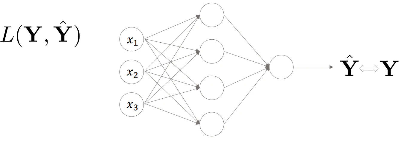
- 誤差(損失)計算
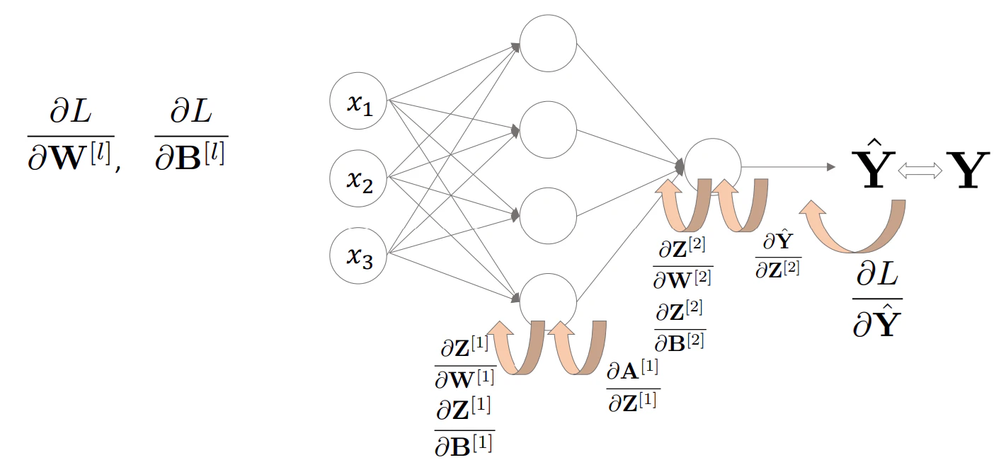
- 誤差逆伝搬
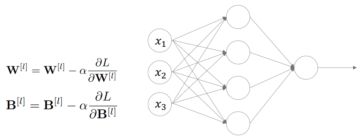
※大体は最急降下法で最適なパラメータを模索する
- 重みの更新
▶誤差逆伝搬とは
- 出力層から入力層にわたって誤差を伝播させていく
- 最終的な結果から出力層 ⇒ 隠れ層 ⇒ 入力層という順番に誤差項$\delta$ を伝播させていく
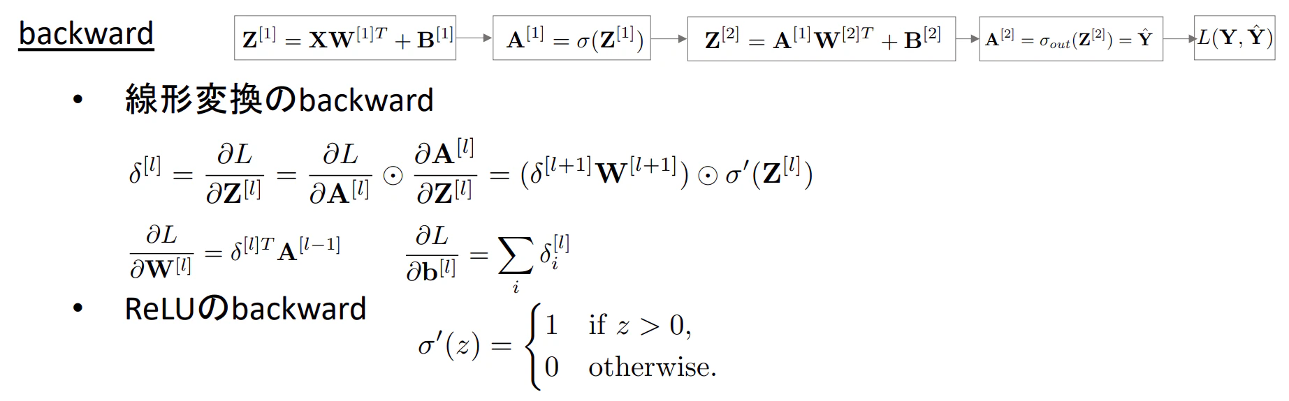
※一般化した$l$層での誤差逆伝播の式は下記のようになる
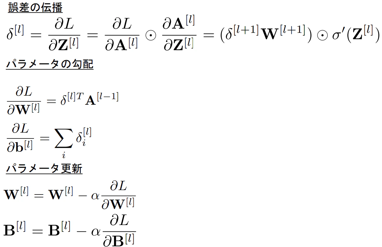
※⦿:各要素毎の積を表す
Pythonで誤差逆伝播をスクラッチ実装
※前提として、Pytorchでは誤差逆伝播を自動で計算してくれるライブラリがあるので、中でどのような動きをしているか想像するのに活用してください。
import torch
from sklearn import datasets
import matplotlib.pyplot as plt
from torch.nn import functional as F
from sklearn.model_selection import train_test_split
import numpy as np

def linear_backward(A, W, b, Z):
    W.grad_ = Z.grad_.T @ A
    b.grad_ = torch.sum(Z.grad_, dim=0) # バイアス項は全てのデータに加算される形になるので,逆伝播時には集約する
    A.grad_ = Z.grad_ @ W

def relu_backward(Z, A):
    # 入力が正なら1(True)として,負なら0(False), それぞれの要素をマスクする
    Z.grad_ = A.grad_ * (Z>0).float()

# softmaxとcrossentropyを同じ関数にする(する必要はないが,pytorchの実装に合わせている
def softmax_cross_entropy(x, y_true):
    e_x = torch.exp(x - torch.max(x, dim=-1, keepdim=True)[0])
    softmax_out =  e_x / (torch.sum(e_x, dim=-1, keepdim=True) + 1e-10)
    loss = -torch.sum(y_true * torch.log(softmax_out + 1e-10)) / y_true.shape[0]
    return loss, softmax_out

def linear(X, W, b):
    return X@W.T + b

def relu(Z):
    return Z.clamp_min(0.)

def forward_and_backward(X, y):
    # forward
    Z1 = linear(X, W1, b1)
    Z1.retain_grad()
    A1 = relu(Z1)
    A1.retain_grad()
    Z2 = linear(A1, W2, b2)
    Z2.retain_grad()
    loss, A2 = softmax_cross_entropy(Z2, y)

    # backward
    Z2.grad_ = (A2 - y) / X.shape[0]
    linear_backward(A1, W2, b2, Z2)
    relu_backward(Z1, A1)
    linear_backward(X, W1, b1, Z1)
    return loss, Z1, A1, Z2, A2
Autogradの結果と比較
- MNISTデータを使用して、スクラッチで実装したbackwardの計算とautogradの結果が等しくなることを確認する
# 1. データロード
dataset = datasets.load_digits()
images = dataset['images']
target = dataset['target']

# 学習データと検証データ分割
X_train, X_val, y_train, y_val = train_test_split(images, target, test_size=0.2, random_state=42)

# 前処理
# 2-1.ラベルのone-hot encoing
y_train = F.one_hot(torch.tensor(y_train), num_classes=10)
X_train = torch.tensor(X_train, dtype=torch.float32).reshape(-1, 64)

y_val = F.one_hot(torch.tensor(y_val), num_classes=10)
X_val = torch.tensor(X_val, dtype=torch.float32).reshape(-1, 64)

# 2-2. 画像の標準化
X_train_mean = X_train.mean()
X_train_std = X_train.std()
X_train = (X_train - X_train_mean) / X_train_std
X_val = (X_val - X_train_mean) / X_train_std

# パラメータの初期化
m, n = X_train.shape
nh = 30
class_num = 10

# パラメータの初期化
# W1 = torch.randn((nh, n), requires_grad=True) # 出力 x 入力
# Kaiming初期化を使って,softmaxの入力が大きくならないようにする
W1 = torch.randn((nh, n)) * torch.sqrt(torch.tensor(2./n))
W1.requires_grad = True
b1 = torch.zeros((1, nh), requires_grad=True) # 1 x nh
# W2 = torch.randn((class_num, nh), requires_grad=True) # 出力 x 入力
# Kaiming初期化を使って,softmaxの入力が大きくならないようにする
W2 = torch.randn((class_num, nh)) * torch.sqrt(torch.tensor(2./nh))
W2.requires_grad = True
b2 = torch.zeros((1, class_num), requires_grad=True) # 1 x nh

# スクラッチのbackward
loss, Z1, A1, Z2, A2 = forward_and_backward(X_train, y_train)

# PytorchのAutograd
loss.backward()

# autogradと大体等しいことを確認
# print(torch.allclose(W1.grad_, W1.grad))
# print(torch.allclose(b1.grad_, b1.grad))
# print(torch.allclose(W2.grad_, W2.grad))
# print(torch.allclose(b2.grad_, b2.grad))  ...4つともすべてTrueになっているか?
誤差逆伝播をMPLに実装
learning_rate = 0.03
batch_size = 30
num_batches = np.ceil(len(y_train) / batch_size).astype(int)
loss_log = []
# 3. パラメータの初期化
W1 = torch.randn((nh, n)) * torch.sqrt(torch.tensor(2./n))
W1.requires_grad = True
b1 = torch.zeros((1, nh), requires_grad=True) # 1 x nh
W2 = torch.randn((class_num, nh)) * torch.sqrt(torch.tensor(2./nh))
W2.requires_grad = True
b2 = torch.zeros((1, class_num), requires_grad=True) # 1 x nh
# ログ
train_losses = []
val_losses = []
val_accuracies = []
# 5. for文で学習ループ作成
epochs = 30
for epoch in range(epochs):
shuffled_indices = np.random.permutation(len(y_train))
running_loss = 0
for i in range(num_batches):
# mini batch作成
start = i * batch_size
end = start + batch_size
batch_indices = shuffled_indices[start:end]
# 6. 入力データXおよび教師ラベルのYを作成
y_true_ = y_train[batch_indices, :] # データ数xクラス数
X = X_train[batch_indices, :] # データ数 x 特徴量数
# import pdb; pdb.set_trace()
# 7. Z計算
Z1 = linear(X, W1, b1)
A1 = relu(Z1)
Z2 = linear(A1, W2, b2)
loss, A2 = softmax_cross_entropy(Z2, y_true_)
# 8. softmaxで予測計算
# y_pred = softmax(Z)
# 9. 損失計算
loss_log.append(loss.item())
running_loss += loss.item()
# 10. 勾配計算
Z2.grad_ = (A2 - y_true_) / X.shape[0]
linear_backward(A1, W2, b2, Z2)
relu_backward(Z1, A1)
linear_backward(X, W1, b1, Z1)
# 11. パラメータ更新
with torch.no_grad():
W1 -= learning_rate * W1.grad_ # .grad -> .grad_
W2 -= learning_rate * W2.grad_ # .grad -> .grad_
b1 -= learning_rate * b1.grad_
b2 -= learning_rate * b2.grad_
# 12. 勾配初期化
W1.grad_ = None
W2.grad_ = None
b1.grad_ = None
b2.grad_ = None
# validation
with torch.no_grad():
Z1_val = linear(X_val, W1, b1)
A1_val = relu(Z1_val)
Z2_val = linear(A1_val, W2, b2)
val_loss, A2_val = softmax_cross_entropy(Z2_val, y_val)
val_accuracy = torch.sum(torch.argmax(A2_val, dim=-1) == torch.argmax(y_val, dim=-1)) / y_val.shape[0]
train_losses.append(running_loss/num_batches)
val_losses.append(val_loss.item())
val_accuracies.append(val_accuracy.item())
# 13. 損失ログ出力
# print(f'epoch: {epoch+1}: train loss:{running_loss/num_batches}, val loss: {val_loss.item()}, val accuracy: {val_accuracy.item()}')
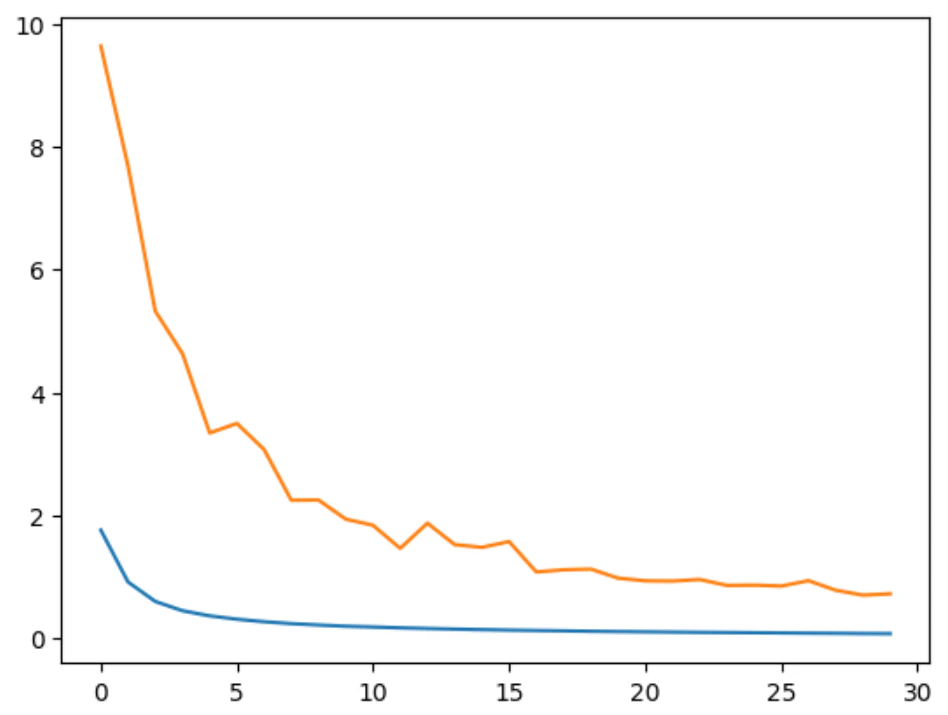
# 経過の描画
plt.plot(train_losses)
plt.plot(val_losses)
▶回帰モデルの誤差逆伝播
- 回帰モデルになったからといっても分類同様の計算を活用できるが、下記のような変化を見せる
‐ 最終層の活性化関数:softmax -> 恒等関数(つまり何もしない)
‐ 損失関数:CE(Cross Entropy) -> MSE(Mean Squere Error)
Pythonで回帰モデルの誤差逆伝播
- 回帰2層NNモデルのforwardとbackwardをスクラッチで実装する
# one-hotしたデータを元に戻す
y_train_reg = torch.argmax(y_train, dim=-1)

def mse(X, y):
    return (X[:, 0] - y).pow(2).mean()

def forward_and_backward(X, y):
    # forward
    Z1 = linear(X, W1, b1)
    Z1.retain_grad()
    A1 = relu(Z1)
    A1.retain_grad()
    Z2 = linear(A1, W2, b2)
    Z2.retain_grad()
    # loss, A2 = softmax_cross_entropy(Z2, y) -> MSE
    loss = mse(Z2, y)

    # backward
    # Z2.grad_ = (A2 - y) / X.shape[0] -> MSE
    Z2.grad_ = 2 * (Z2 - y.unsqueeze(dim=-1)) / X.shape[0]
    linear_backward(A1, W2, b2, Z2)
    relu_backward(Z1, A1)
    linear_backward(X, W1, b1, Z1)
    return loss, Z1, A1, Z2, A2

# パラメータの初期化
m, n = X_train.shape
nh = 30

W1 = torch.randn((nh, n), requires_grad=True) # 出力 x 入力
b1 = torch.zeros((1, nh), requires_grad=True) # 1 x nh

W2 = torch.randn((1, nh), requires_grad=True) # 出力 x 入力
b2 = torch.zeros((1, 1), requires_grad=True) # 1 x 1
loss, Z1, A1, Z2, A2 = forward_and_backward(X_train, y_train_reg)
loss.backward()

# autogradとおおよそ等しいことを確認、以下全てTureになっているか
# print(torch.allclose(W1.grad_, W1.grad))
# print(torch.allclose(b1.grad_, b1.grad))
# print(torch.allclose(W2.grad_, W2.grad))
# print(torch.allclose(b2.grad_, b2.grad))
今までのコードをRefactoring
# ======モデル======
class Linear():
    def __init__(self, in_features, out_features):
        self.W = torch.randn((out_features, in_features)) * torch.sqrt(torch.tensor(2.0 / in_features))
        self.W.requires_grad = True
        self.b = torch.zeros((1, out_features), requires_grad=True)

    def forward(self, X):
        self.X = X
        self.Z = X @ self.W.T + self.b
        return self.Z

    def backward(self, Z):
        self.W.grad_ = Z.grad_.T @ self.X
        self.b.grad_ = torch.sum(Z.grad_, dim=0)
        self.X.grad_ = Z.grad_ @ self.W
        return self.X.grad_

class ReLU():
    def forward(self, X):
        self.X = X
        return X.clamp_min(0.)

    def backward(self, A):
        return A.grad_ * (self.X > 0).float()

class SoftmaxCrossEntropy:
    def forward(self, X, y):
        e_x = torch.exp(X - torch.max(X, dim=-1, keepdim=True)[0])
        self.softmax_out = e_x / (torch.sum(e_x, dim=-1, keepdim=True) + 1e-10)

        log_probs = torch.log(self.softmax_out + 1e-10)
        target_log_probs = log_probs * y

        self.loss = -target_log_probs.sum(dim=-1).mean()
        return self.loss

    def backward(self, y):
        return (self.softmax_out - y) / y.shape[0]

class Model:
    def __init__(self, input_features, hidden_units, output_units):
        self.linear1 = Linear(input_features, hidden_units)
        self.relu = ReLU()
        self.linear2 = Linear(hidden_units, output_units)
        self.loss_fn = SoftmaxCrossEntropy()

    def forward(self, X, y):
        self.X = X
        self.Z1 = self.linear1.forward(X)
        self.A1 = self.relu.forward(self.Z1)
        self.Z2 = self.linear2.forward(self.A1)
        self.loss = self.loss_fn.forward(self.Z2, y)
        return self.loss, self.Z2

    def backward(self, y):
        self.Z2.grad_ = self.loss_fn.backward(y)
        self.A1.grad_ = self.linear2.backward(self.Z2)
        self.Z1.grad_ = self.relu.backward(self.A1)
        self.X.grad_ = self.linear1.backward(self.Z1)

    def zero_grad(self):
        # 勾配の初期化
        self.linear1.W.grad_ = None
        self.linear1.b.grad_ = None
        self.linear2.W.grad_ = None
        self.linear2.b.grad_ = None

    def step(self, learning_rate):
        # パラメータの更新
        self.linear1.W -= learning_rate * self.linear1.W.grad_
        self.linear1.b -= learning_rate * self.linear1.b.grad_
        self.linear2.W -= learning_rate * self.linear2.W.grad_
        self.linear2.b -= learning_rate * self.linear2.b.grad_

## Refactoring後の学習ループ(OptimizerやDataset, Dataloaderは後ほどRefactoring)
# ===データの準備====
dataset = datasets.load_digits()
data = dataset['data']
target = dataset['target']
images = dataset['images']
X_train, X_val, y_train, y_val = train_test_split(images, target, test_size=0.2, random_state=42)
x_train_mean = X_train.mean()
x_train_std = X_train.std()
X_train = (X_train - x_train_mean) / x_train_std
X_val = (X_val - x_train_mean) / x_train_std
X_train = torch.tensor(X_train.reshape(-1, 64), dtype=torch.float32)
X_val = torch.tensor(X_val.reshape(-1, 64), dtype=torch.float32)
y_train = F.one_hot(torch.tensor(y_train), num_classes=10) #1437 x 10
y_val = F.one_hot(torch.tensor(y_val), num_classes=10) # 360 x 10
batch_size = 30
# モデルの初期化
model = Model(input_features=64, hidden_units=10, output_units=10)

learning_rate = 0.01

# ログ
train_losses = []
val_losses = []
val_accuracies = []
for epoch in range(100):
    # エポック毎にデータをシャッフル
    shuffled_indices = np.random.permutation(len(y_train))
    num_batches = np.ceil(len(y_train)/batch_size).astype(int)
    running_loss = 0.0

    for i in range(num_batches):

        # mini batch作成
        start = i * batch_size
        end = start + batch_size

        batch_indices = shuffled_indices[start:end]
        y_true_ = y_train[batch_indices, :] # batch_size x 10
        X = X_train[batch_indices] # batch_size x 64

        # 順伝播と逆伝播の計算
        loss, _ = model.forward(X, y_true_)
        model.backward(y_true_)
        running_loss += loss.item()

        # パラメータ更新
        with torch.no_grad():
            model.step(learning_rate)

        model.zero_grad()

    # validation
    with torch.no_grad():
        val_loss, Z2_val = model.forward(X_val, y_val)

        val_accuracy = torch.sum(torch.argmax(Z2_val, dim=-1) == torch.argmax(y_val, dim=-1)) / y_val.shape[0]

    train_losses.append(running_loss/num_batches)
    val_losses.append(val_loss.item())
    val_accuracies.append(val_accuracy)
    # print(f'epoch: {epoch}: train error: {running_loss/num_batches}, validation error: {val_loss.item()}, validation accuracy: {val_accuracy}')