Python初心者の備忘録 #25 ~深層学習超入門編01~

はじめに

今回私は最近はやりのchatGPTに興味を持ち、深層学習について学んでみたいと思い立ちました！
深層学習といえばPythonということなので、最終的にはPythonを使って深層学習ができるとこまでコツコツと学習していくことにしました。
ただ、勉強するだけではなく少しでもアウトプットをしようということで、備忘録として学習した内容をまとめていこうと思います。
この記事が少しでも誰かの糧になることを願っております！
※投稿主の環境はWindowsなのでMacの方は多少違う部分が出てくると思いますが、ご了承ください。
最初の記事：Python初心者の備忘録 #01
前の記事：Python初心者の備忘録 #24 ~機械学習入門編10~
次の記事：まだ

今回はPytorch、Tensor、Tensorでのロジスティック回帰・多項ロジスティック回帰、Mini-batch学習についてまとめております。

■学習に使用している資料

Udemy：①米国AI開発者がやさしく教える深層学習超入門第一弾【Pythonで実践】

■事前準備

▶Dockerfile

深層学習用の仮想環境を準備するためにDockerfile、docker-compose.ymlをそれぞれ指定の通りに修正してください。

Dockerfile

FROM ubuntu:latest 
# update
RUN apt-get -y update && apt-get install -y \
graphviz \
libsm6 \
libxext6 \
libxrender-dev \
libglib2.0-0 \
sudo \
wget \
vim

#install anaconda3
WORKDIR /opt
# download anaconda package and install anaconda
# archive -> https://repo.anaconda.com/archive/
RUN wget https://repo.anaconda.com/archive/Anaconda3-2022.10-Linux-x86_64.sh && \
sh /opt/Anaconda3-2022.10-Linux-x86_64.sh -b -p /opt/anaconda3 && \
rm -f Anaconda3-2022.10-Linux-x86_64.sh
# set path
ENV PATH /opt/anaconda3/bin:$PATH

# update pip and install pxackages
RUN pip install --upgrade pip && \
	pip install --upgrade scikit-learn && \
    pip install opencv-python && \
    pip install nibabel && \
    pip install --upgrade plotly && \
    pip install chart_studio && \
    pip install jupyter-dash && \
    pip install --upgrade "ipywidgets>=7.6" && \
    pip install lightgbm && \
    pip install xgboost && \
    pip install graphviz && \
    pip install catboost && \
    pip install category_encoders && \
    pip install hyperopt && \
    pip install hpsklearn


WORKDIR /
RUN mkdir /work

# execute jupyterlab as a default command
CMD ["jupyter", "lab", "--ip=0.0.0.0", "--allow-root", "--LabApp.token=''"]

docker-compose.yml

services:  
  basic:    
    build:      
      context: .      
      dockerfile: Dockerfile    
    image: datascientistus/dl-python-env   
    container_name: ds-python    
    ports:      
      - "8888:8888"    
    volumes:      
      - "/c/Users/ytati/Desktop/work:/work"    
    restart: on-failure

■PytorchとTensor

▶Pytorchとは

• 深層学習のためのオープンソースフレームワークで他のフレームワークではできない様な柔軟なカスタマイズができる
• 以前はTensorFlowがよくつかわれていたのだが、今はPytorchのほうが強い

▶Tensorとは

• PytorchやTensorFlowで使われる多次元配列のこと
• 深層学習の計算の核となるようなデータ構造でNumpy Arrayのようなもの
• Numpy Arrayとの違いは「GPUによる計算の高速化」と「自動微分(Auto Grad)」が可能

▶PythonでTensorの作成

• import torchでPytorchをimport
• torch.tensor()にlistを入れることでtensorを作成
  • デフォルトの要素のデータ型はfloat32なので、データ型を意識して作成するとこが重要
  • dtype引数を使ってデータ型を指定(例:dtype=torch.float64)
• numpy関数との類似関数
  • torch.zeros() : np.zeros()
  • torch.ones() : np.ones()
  • torch.eye() : np.eye()
  • torch.rand() : np.random.rand()
• .shape()でtensorのshapeを表示
  ※リスト表示でprintされるが、実際はtuple同様の不変オブジェクト

# Pytorchをimport
import torch
import numpy as np
# 乱数の種の固定が可能
torch.manual_seed(42)

# tensorを作成
my_list = [1, 2, 3, 4]
tensor_from_list = torch.tensor(my_list)
print("Tensor from list:", tensor_from_list) # => Tensor from list: tensor([1, 2, 3, 4])

type(tensor_from_list) # => torch.Tensor

# intのリストで作成したTensorのデータ形はint64になる(デフォルトはfloat32)
tensor_from_list.dtype # => torch.int64

# floatのlistで作ったtensorはfloat32
my_list = [1., 2., 3., 4.]
tensor_from_list = torch.tensor(my_list)
print("Tensor from list:", tensor_from_list) # => Tensor from list: tensor([1., 2., 3., 4.])
tensor_from_list.dtype # => torch.float32

# dtype引数でデータ型を指定
tensor_from_list = torch.tensor(my_list, dtype=torch.float64)
tensor_from_list # => tensor([1., 2., 3., 4.], dtype=torch.float64)

# Tensorのshapeを表示
zeros_tensor = torch.zeros((2, 3))
zeros_tensor.shape # => torch.Size([2, 3])

▶PythonでTensor操作と便利関数

tensor操作

• torch.permute() : np.transpose()
  ※torch.tranpose()は，2軸を入れ替える関数、2次元のtensorであれば.Tや.t()で転置可能
• torch.reshape() : np.reshape()
  ※torch.view()も同様にreshapeするがメモリが連続の場合のみ
• torch.flaKen() : .flaKen()
• torch.squeeze() : np.squeeze()
• torch.unsqueeze() : np.expand_dims()

tensorの便利関数

• torch.sum() : np.sum()
• torch.mean() : np.mean()
• torch.std() : np.std()
• torch.sqrt() : np.sqrt()

numpyと違い、Pytorchでの上記関数の戻り値はtensorなので注意
※値だけほしい場合は.item()を最後につける

.reshape()や.view()の挙動について

.reshape()で作成した変数はコピーを作成しているのではなく、メモリ上のアドレスをコピーしている。なので、reshape後の変数を修正すると、reshape前の変数も変わってしまう。

tensor_example = torch.rand((2, 3, 4))
print(tensor_example)
"""
tensor([[[0.1189, 0.5576, 0.2109, 0.9298],
         [0.7667, 0.8001, 0.2030, 0.6653],
         [0.9902, 0.0712, 0.9342, 0.5196]],

        [[0.0742, 0.1989, 0.3927, 0.8927],
         [0.2684, 0.5062, 0.5581, 0.7075],
         [0.0618, 0.6984, 0.2023, 0.3045]]])
"""

# reshape
tensor_reshaped = torch.reshape(tensor_example, (6, 4))
print(tensor_reshaped)
"""
tensor([[0.1189, 0.5576, 0.2109, 0.9298],
        [0.7667, 0.8001, 0.2030, 0.6653],
        [0.9902, 0.0712, 0.9342, 0.5196],
        [0.0742, 0.1989, 0.3927, 0.8927],
        [0.2684, 0.5062, 0.5581, 0.7075],
        [0.0618, 0.6984, 0.2023, 0.3045]])
"""

# tensor_reshapedを変更
tensor_reshaped[0] = 0

# tendor_exampleの値も変わる -> メモリを使いまわしている
print(tensor_example)
"""
tensor([[[0.0000, 0.0000, 0.0000, 0.0000],
         [0.7667, 0.8001, 0.2030, 0.6653],
         [0.9902, 0.0712, 0.9342, 0.5196]],

        [[0.0742, 0.1989, 0.3927, 0.8927],
         [0.2684, 0.5062, 0.5581, 0.7075],
         [0.0618, 0.6984, 0.2023, 0.3045]]])
"""

ただし、このようになるのはreshape対象のtensorがメモリ上で連続した場所に格納されている場合で、非連続なtensorの場合メモリのアドレスではなく、純粋にコピーを作成する。

# メモリが連続でなければreshape後のtensorはコピーを返す
# 連続的なメモリレイアウトを持つTensorを作成
x = torch.tensor([[1, 2], [3, 4], [5, 6]])

# 連続的なメモリレイアウトを持たない部分Tensorを取得 (transposed tensor)
y = x.T

# y は非連続的なメモリレイアウトを持つことを確認
print(y.is_contiguous())  # => False

# reshape を使用して y の形状を変更
z = y.reshape(-1)
# 以下はエラーになる(.view()はメモリ上連続なtensorにのみ使用可能)
# メモリを節約したい場合は.view()を利用するといい
# z = y.view(-1)

# z が y とメモリを共有していないことを確認 (コピーが作成されたことを意味する)
print(z.data_ptr() == y.data_ptr())  # => False

▶行列の計算

加減算および要素毎の剰除算

• Numpyと同様で+, -, *, /

行列の積

• torch.mm()、torch.matmul()もしくは@演算子を使用
  • Numpy Arrayではnp.dot()または@演算子を使用
  • torch.dot()は1次元に対してのみドット積(ベクトルの内積)を計算

# 3x3のTensorを作成
a = torch.rand((3, 3))
b = torch.rand((3, 3))

# 加減算および要素毎の剰除算
add = a + b
sub = a - b
mul = a * b
div = a / b

# 行列の積
mm = torch.mm(a, b)
matmul = torch.matmul(a, b)
at_op = a @ b

行列の積がわからない場合は下記サイトを参照してください。
https://lab-brains.as-1.co.jp/enjoy-learn/2023/07/50258/

▶Broadcasting

• 演算する2つのtensorが同じ次元でない場合、次元の少ない方が次元を増やして演算が可能にする
• ルール
  • rank数(次元)が少ない方の配列のshapeの左側にサイズ1の次元を追加する
    例：(2, 3) -> (1, 2, 3)
  • shapeの右側からサイズ数(値)を比較し、数が一致するか、サイズが1であればブロードキャスティング可能
  • サイズ1の次元がもう一方の次元のサイズに拡大する

# (3, 3)とスカラーの演算
a = torch.rand((3, 3))
scalar = 5
result1 = a + scalar
"""
a
tensor([[0.6440, 0.7071, 0.6581],
        [0.4913, 0.8913, 0.1447],
        [0.5315, 0.1587, 0.6542]])

result1
tensor([[5.6440, 5.7071, 5.6581],
        [5.4913, 5.8913, 5.1447],
        [5.5315, 5.1587, 5.6542]])
"""

# (3, 3)と(1, 3)の演算
b = torch.rand((1, 3))
result2 = a + b
print(b)
print(result2)
"""
b
tensor([[0.3278, 0.6532, 0.3958]])

result2
tensor([[0.9718, 1.3603, 1.0540],
        [0.8191, 1.5445, 0.5406],
        [0.8593, 0.8119, 1.0500]])
"""

# (32, 128, 128, 3)と(128, 128, 3)の演算
c = torch.rand((32, 128, 128, 3))
d = torch.rand((128, 128, 3))
result3 = c + d
print(result3.shape)  # -> torch.Size([32, 128, 128, 3])

# (32, 128, 128, 3)と(128, 128, 6)の演算は形状が不一致なためエラー
c = torch.rand((32, 128, 128, 3))
d = torch.rand((128, 128, 6))
# 以下はエラー
# result3 = c + d 

# (1, 128, 128, 3)と(8, 128, 128, 1)の演算
e = torch.rand((1, 128, 128, 3))
f = torch.rand((8, 128, 128, 1))
result4 = e + f
print(result4.shape)  # -> torch.Size([8, 128, 128, 3])

■ロジスティック回帰からニューラルネットワークへ

必要に応じて下記記事で内容を復習してください。

• ロジスティック回帰
• 最急降下法

本記事では深層学習におけるロジスティック回帰の式を下記のように表す

さらに、ベクトル表記と行列表記は下記のようにする(※$^T$は転置を表す)

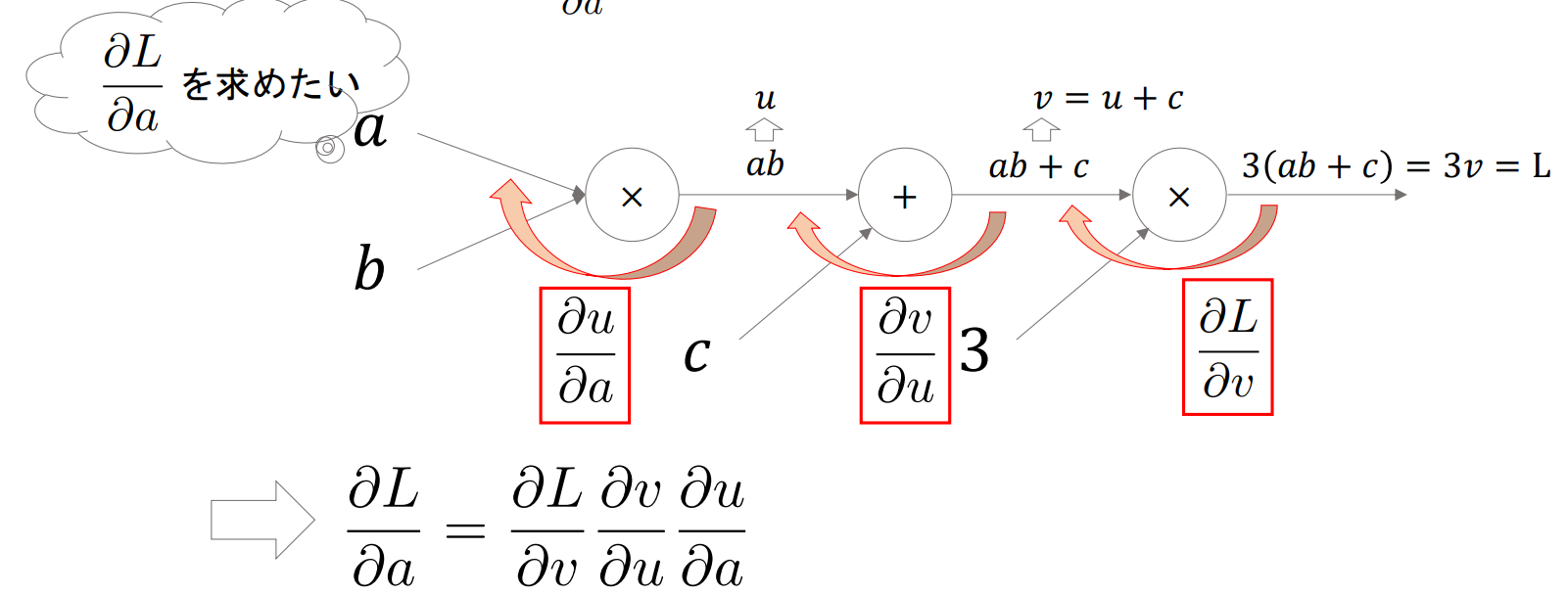
▶計算グラフ(Computational Graph)

• 計算過程をグラフ構造として表現したもので、Pytorchでは内部で計算グラフを構成している(Autograd:自動微分)
• これによって任意の計算グラフの勾配を計算することができる

• 基本的に「末端ノード(a, b)についての最終出力(L)の(偏)微分」を求める

例：$\frac{\partial L}{\partial a}$を求める場合

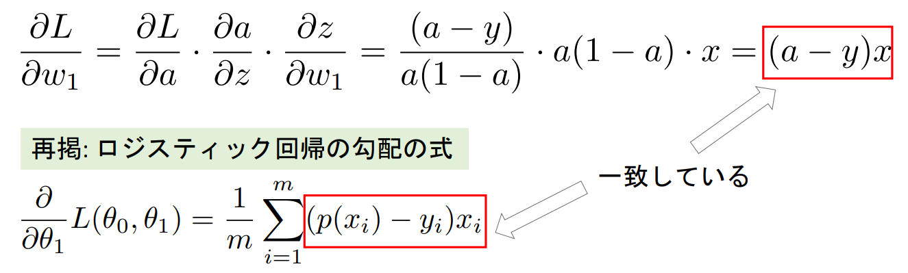
▶損失関数の計算グラフ

• 損失関数を計算グラフで表すと下記のようになる

• 損失関数は$w_1$と$b$によって変動するので、それぞれ$\frac{\partial L}{\partial w_1}$と$\frac{\partial L}{\partial b}$を求めると下記のようになる
  • $\frac{\partial L}{\partial w_1} = (a-y)x$ ※ロジスティック回帰の勾配の式と一致しているのがわかる
  • $\frac{\partial L}{\partial b}=(a-y)$

▶Autograd(自動微分)

• pytorchでは計算グラフを自動的に構築し、勾配を逆方向に計算する
  • tensor生成時にrequires_grad=Trueを設定することで自動微分を有効にする
  • 計算後に.backward()を呼ぶことで自動的に勾配が計算される
• 勾配情報は.grad属性に累積されるが、末端ノードに対する勾配しか保存されない
  • 中間ノードに対する勾配を保存したい場合は当該tensorに対して.retain_grad()を実行する

例：$z=ylog(x)+sin(y)$の$\frac{\partial z}{\partial x}$と$\frac{\partial z}{\partial y}$を求める。ただし、初期のtensorの値は$x=2,y=3$とする。

# xとyの値を設定し、requires_grad=Trueで微分可能にする
x = torch.tensor(2., requires_grad=True)
y = torch.tensor(3., requires_grad=True)

# 出力関数
z = y * torch.log(x) + torch.sin(y)

# zに対して微分を計算
z.backward()

# 偏微分 dz/dy と dz/dx を取得
dz_dx = x.grad
dz_dy = y.grad

print("dz/dx:", dz_dx) # -> dz/dx: tensor(1.5000) (※y/xと同じ)
print("dz/dy:", dz_dy) # -> dz/dy: tensor(-0.2968) (※torch.log(x) + torch.cos(y)と同じ)

中間ノードの勾配

例：$z=(x+y)^2$の中間ノード$\frac{\partial z}{\partial (x+y)}$を求める。ただし、初期のtensorの値は$x=2,y=3$とする。

# 入力変数
x = torch.tensor(2., requires_grad=True)
y = torch.tensor(3., requires_grad=True)

# 中間ノード（合計）
sum_xy = x + y
sum_xy.retain_grad()  # この中間ノードの勾配を保存するためにretain_grad()を使用

# 出力関数
z = sum_xy ** 2

# 勾配を計算
z.backward()

# 各変数の勾配を表示
print("df/dx:", x.grad.item())  # -> df/dx: 10.0
print("df/dy:", y.grad.item())  # -> df/dy: 10.0
 # 中間ノードの勾配
print("df/d(sum_xy):", sum_xy.grad.item())  # -> df/d(sum_xy): 10.0

自動微分の無効化

• 勾配の計算が必要ない場合は、with torch.no_grad():内に関数を記載することで自動微分を無効化することができる
  • 計算速度の向上、メモリの節約が期待できる
  • モデルの推論(予測)時やパラメータの更新時に使用する

x = torch.tensor(2., requires_grad=True)
y = torch.tensor(3., requires_grad=True)

with torch.no_grad():
    z1 = y * torch.log(x) + torch.sin(y)

z2 = y * torch.log(x) + torch.sin(y)

# 逆伝播
# 以下はエラー．with torch.no_grad()内の計算では勾配は保持されない
# z1.backward()
z2.backward()

# 勾配が計算されていることを確認
print(y.grad)  # -> tensor(-0.2968)

■多項ロジスティック回帰とニューラルネットワーク

必要に応じて下記記事で内容を復習してください。

• 多項ロジスティック回帰

▶MNISTデータセットで多項ロジスティック回帰

MNISTとは
手書きの数字(0~9)のデータ(10クラス)
それぞれのpixel値を特徴量として扱う(8 x 8 = 64個の特徴量)

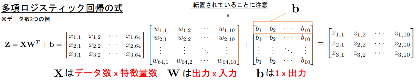
• 多項ロジスティック回帰の式は下記のようなイメージ
  ※$b$はもともと「$1×n$」のベクトルだが、ブロードキャストされて「$データ数×n$」に拡張されている

• 実際にスクラッチで実装する場合の手順例は下記のようになる

1. データロード
   ・sklearn.datasets.load_digits()
2. 前処理
   ・ラベルのone-hot encoding：torch.nn.functional.one_hot()
   ・画像の標準化
3. パラメータ初期化
   ・torch.rand(requires_grad=True)
4. 損失関数とsoftmax関数実装
5. for文で学習ループ作成(5回) (ループの単位をepochという)
6. 入力データ$X$および教師ラベル$Y$作成 (1データずつ処理)
7. 出力結果$Z$計算
8. softmaxで予測計算
9. 損失計算
10. 勾配計算
11. パラメータ更新
12. 勾配初期化
    ・.grad.zero_()
    ※Pytorchでは_()というように最後にアンダースコアをつけて関数を呼び出すとその結果を呼び出し元に代入してくれる。(W.grad.zero_()：W.grad = 0)
13. 損失ログ出力

softmaxと交差エントロピーの実装において
それぞれ実装時に下記のような工夫が必要

import numpy as np
import torch
from torch.nn import functional as F
from sklearn import datasets
from sklearn.model_selection import train_test_split
import matplotlib.pyplot as plt

# 1. データロード
dataset = datasets.load_digits()
images = dataset['images']  # 学習データ
target = dataset['target']  # 正解ラベル：array([0, 1, 2, ..., 8, 9, 8])

# データ可視化
plt.imshow(images[2], cmap='gray')
print(images.shape)

# 2. 前処理
# 2-1.ラベルのone-hot encoing
y_true = F.one_hot(torch.tensor(target), num_classes=10)

# NumPyのデフォルトはfloat64, torchはfloat32で，演算時にエラーになるのでfloat32に揃える
images = torch.tensor(images, dtype=torch.float32).reshape(-1, 64)

# 2-2. 画像の標準化
images = (images - images.mean()) / images.std()
learning_rate = 0.03  # 学習率
loss_log = []  # 損失保存用

# 3. パラメータの初期化
W = torch.rand((10, 64), requires_grad=True) # 出力 x 入力
b = torch.rand((1, 10), requires_grad=True) # 1 x 出力

# 4. softmaxとcross entropy
def softmax(x):
    e_x = torch.exp(x - torch.max(x, dim=-1, keepdim=True)[0])
    return e_x / (torch.sum(e_x, dim=-1, keepdim=True) + 1e-10)

def cross_entropy(y_true, y_pred):
    return -torch.sum(y_true * torch.log(y_pred + 1e-10)) / y_true.shape[0]
    
# 5. for文で学習ループ作成
for epoch in range(5):
    running_loss = 0
    for i in range(len(target)):
        # 6. 入力データXおよび教師ラベルのYを作成
        y_true_ = y_true[i].reshape(-1, 10) # データ数xクラス数
        X = images[i].reshape(-1, 64) # データ数 x 特徴量数

        # 7. Z計算
        Z = X@W.T + b

        # 8. softmaxで予測計算
        y_pred = softmax(Z)

        # 9. 損失計算
        loss = cross_entropy(y_true_, y_pred)
        loss_log.append(loss.item())
        running_loss += loss.item()
        
        # 10. 勾配計算
        loss.backward()

        # 11. パラメータ更新
        with torch.no_grad():
            W -= learning_rate * W.grad
            b -= learning_rate * b.grad

        # 12. 勾配初期化
        W.grad.zero_()
        b.grad.zero_()

    # 13. 損失ログ出力
    print(f'epoch: {epoch+1}: {running_loss/len(target)}')

    """ 出力結果
    epoch: 1: 0.4074933143537554
    epoch: 2: 0.14019991623049766
    epoch: 3: 0.1081952229690629
    epoch: 4: 0.09146877579146422
    epoch: 5: 0.08023116896337683
    """

# 学習したモデルで全データのaccuracyを計算する（学習に使っているデータに対してのAccuracyであることに注意）
X = torch.tensor(images, dtype=torch.float32)
Z = X@W.T + b
y_pred = softmax(Z)

# accuracy = 正しく分類できた数/全サンプル数
torch.sum(torch.argmax(y_pred, dim=-1) == torch.argmax(y_true, dim=-1)) / y_true.shape[0]  # -> tensor(0.9772)

# 損失の推移を描画
plt.plot(loss_log)

■ミニバッチ(Mini-batch)学習

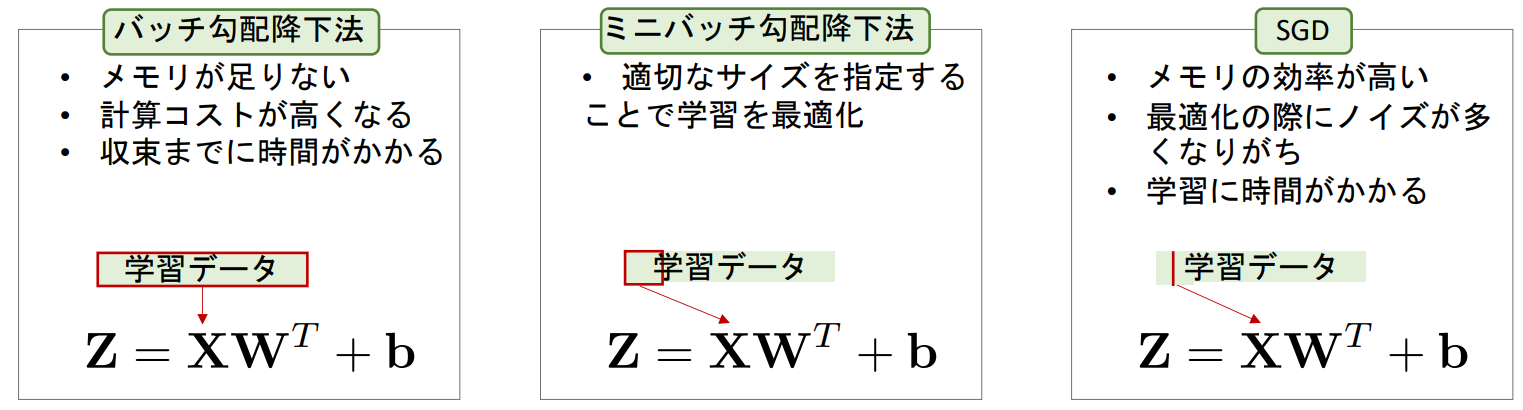
▶ミニバッチ勾配降下法(ミニバッチ学習)

• 全ての学習データを一気に学習させるのではなく、いくつかのデータを1つのミニバッチにして学習していく手法
• ミニバッチのサイズは自由に選択できるが、2の累乗が選ばれることが多い
• ミニバッチサイズが1の場合は確率的勾配降下法(SGD:Stochastic Gradient Descent)といい、全データの場合はバッチ勾配降下法という(※ミニバッチ勾配降下法をSGDと呼ぶ場合もある)

▶バッチサイズの決め方

• 2の累乗にするのが通例で、その他にも下記を考慮して決定する
  • 計算リソース(特にGPUのメモリ)
  • データセットのサイズ：元データの大小によって、バッチサイズも大小する
  • モデルの複雑さ：複雑なモデルはバッチサイズを小さくして計算コストを抑える
  • 安定性と精度：訓練の安定性と汎化性能のトレードオフでバッチサイズが大きければ訓練は安定化し、汎化性能が落ちる
• 現実的にはGPUのメモリに乗る最大の$2^n$のバッチサイズを選ぶことが多い

Pythonでミニバッチ学習

• MINSTを利用したロジスティック回帰の例のコードを下記条件でミニバッチ化する。
  • 毎回のepochの開始時に学習データをシャッフルし、毎回異なるミニバッチ群を作成する
  • 各バッチ毎の損失の平均を累積し、epochの最後に損失の平均を計算する
  • バッチサイズには30を指定

loss_log = []
# バッチサイズを指定
batch_size = 30
# 総バッチ数を計算
num_batches = np.ceil(len(target) / batch_size).astype(int)

# 3. パラメータの初期化
W = torch.rand((10, 64), requires_grad=True) # 出力x入力
b = torch.rand((1, 10), requires_grad=True) # 1 x 出力

# 5. for文で学習ループ作成
for epoch in range(5):
    shuffled_indices = np.random.permutation(len(target))
    running_loss = 0
    for i in range(num_batches):

        # mini batch作成
        start = i * batch_size
        end = start + batch_size
        batch_indices = shuffled_indices[start:end]
        
        # 6. 入力データXおよび教師ラベルのYを作成
        y_true_ = y_true[batch_indices, :] # データ数xクラス数
        X = images[batch_indices, :] # データ数 x 特徴量数
        # ブレークポイントを設置
        # import pdb; pdb.set_trace()

        # 7. Z計算
        Z = X@W.T + b

        # 8. softmaxで予測計算
        y_pred = softmax(Z)

        # 9. 損失計算
        loss = cross_entropy(y_true_, y_pred)
        loss_log.append(loss.item())
        running_loss += loss.item()
        
        # 10. 勾配計算
        loss.backward()

        # 11. パラメータ更新
        with torch.no_grad():
            W -= learning_rate * W.grad
            b -= learning_rate * b.grad

        # 12. 勾配初期化
        W.grad.zero_()
        b.grad.zero_()

    # 13. 損失ログ出力
    # print(f'epoch: {epoch+1}: {running_loss/num_batches}')

X = torch.tensor(images, dtype=torch.float32)
Z = X@W.T + b
y_pred = softmax(Z)
# Accuracy
torch.sum(torch.argmax(y_pred, dim=-1) == torch.argmax(y_true, dim=-1)) / y_true.shape[0]  # -> tensor(0.8976)

▶学習データと検証データに分割しての学習

• sklearn.model_selection.train_test_splitを使用して、手元のデータを学習用と検証用に分割する
• 実際に下記条件で、前章のコードを修正する
  • 学習データと検証データを8:2で分割
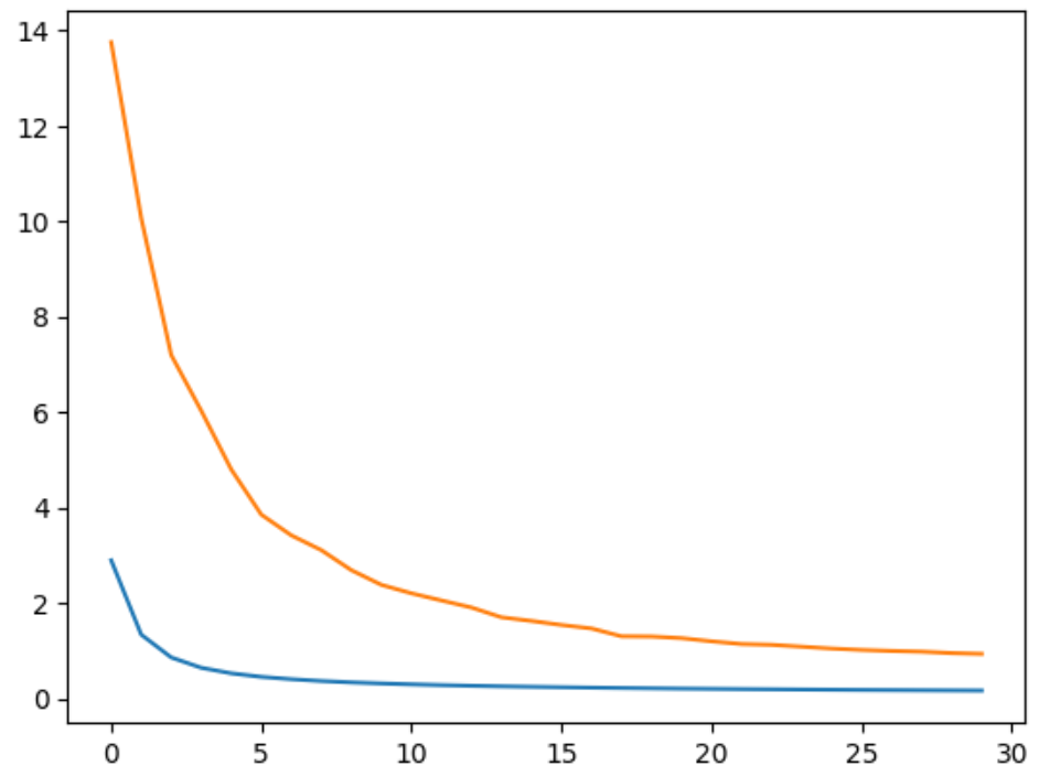
  • それぞれのログを記録し、学習曲線を確認できるようにする
  • 毎epoch毎に検証データでのAccruacyを計算する

# 1. データロード
dataset = datasets.load_digits()
images = dataset['images']
target = dataset['target']

# 学習データと検証データ分割
X_train, X_val, y_train, y_val = train_test_split(images, target, test_size=0.2, random_state=42)

# 前処理
# 2-1.ラベルのone-hot encoing
y_train = F.one_hot(torch.tensor(y_train), num_classes=10)
X_train = torch.tensor(X_train, dtype=torch.float32).reshape(-1, 64)

y_val = F.one_hot(torch.tensor(y_val), num_classes=10)
X_val = torch.tensor(X_val, dtype=torch.float32).reshape(-1, 64)

# 2-2. 画像の標準化
X_train_mean = X_train.mean()
X_train_std = X_train.std()
X_train = (X_train - X_train_mean) / X_train_std
X_val = (X_val - X_train_mean) / X_train_std
# 以下のように手元のデータ全ての平均&標準偏差を使えば，学習データと検証データの分布を近くすることが可能
# しかし，この場合validationの精度は，未知のデータよりも若干高くなることに注意
# X_train = (X_train - images.mean()) / images.std()
# X_val = (X_val - images.mean()) / images.std()

batch_size = 30
num_batches = np.ceil(len(y_train) / batch_size).astype(int)
loss_log = []

# 3. パラメータの初期化
W = torch.rand((10, 64), requires_grad=True) # 出力x入力
b = torch.rand((1, 10), requires_grad=True) # 1 x 出力

# ログ
train_losses = []
val_losses = []
val_accuracies = []

# 5. for文で学習ループ作成
epochs = 30
for epoch in range(epochs):
    shuffled_indices = np.random.permutation(len(y_train))
    running_loss = 0
    for i in range(num_batches):

        # mini batch作成
        start = i * batch_size
        end = start + batch_size
        batch_indices = shuffled_indices[start:end]
        
        # 6. 入力データXおよび教師ラベルのYを作成
        y_true_ = y_train[batch_indices, :] # データ数xクラス数
        X = X_train[batch_indices, :] # データ数 x 特徴量数
        # import pdb; pdb.set_trace()

        # 7. Z計算
        Z = X@W.T + b

        # 8. softmaxで予測計算
        y_pred = softmax(Z)

        # 9. 損失計算
        loss = cross_entropy(y_true_, y_pred)
        loss_log.append(loss.item())
        running_loss += loss.item()
        
        # 10. 勾配計算
        loss.backward()

        # 11. パラメータ更新
        with torch.no_grad():
            W -= learning_rate * W.grad
            b -= learning_rate * b.grad

        # 12. 勾配初期化
        W.grad.zero_()
        b.grad.zero_()
        
    # validation
    with torch.no_grad():
        Z_val = X_val@W.T + b
        y_pred_val = softmax(Z_val)

        val_loss = cross_entropy(y_val, y_pred_val)
        val_accuracy = torch.sum(torch.argmax(y_pred_val, dim=-1) == torch.argmax(y_val, dim=-1)) / y_val.shape[0]

    train_losses.append(running_loss/num_batches)
    val_losses.append(val_loss.item())
    val_accuracies.append(val_accuracy.item())
        
    # 13. 損失ログ出力
    # print(f'epoch: {epoch+1}: train loss:{running_loss/num_batches}, val loss: {val_loss.item()}, val accuracy: {val_accuracy.item()}')

plt.plot(train_losses)
plt.plot(val_losses)

次の記事

まだ