はじめに
今回は自作TrainingLoopを作成してみようと思います。
これを用いると、昨日ご紹介したtf.data.Datasetの実力を発揮することができます。
自作トレーニングループを組む
まずは基本的なことから述べていきます。
基本
注意🚨
TensorFlowのバージョンは2.0で動かしています。基本的にeager modeなので、TF1.15等では動きません。
また、前提としてAdventCalender1日目,2日目,3日目を学んでいる前提なので、
このコードの意味は・・・?🤔となったらまずは振り返りをしていただけると幸いです。
import
import numpy as np
import tensorflow as tf
import tensorflow.keras as keras
import tensorflow_addons as tfa
import matplotlib.pyplot as plt
from tqdm import tqdm
from sklearn.model_selection import train_test_split
ここに書いてあるimportは全て使いますので、忘れずにpipするなりしてください。
modelを用意
実際に計算するDNNのモデルを用意しましょう。
使うモデルはCIFAR-10でaccuracy95%--CNNで精度を上げるテクニック--を参考にいたしました。
class ConvLayer1(keras.layers.Layer):
    def __init__(self, output_filter=64, **kwargs):
        super(ConvLayer1, self).__init__(output_filter, **kwargs)
        self.conv1_1 = keras.layers.Conv2D(output_filter,3,padding="same",activation="relu",kernel_initializer='he_normal')
        self.conv1_2 = keras.layers.Conv2D(output_filter,3,padding="same",activation="relu",kernel_initializer='he_normal')
        self.BN = keras.layers.BatchNormalization()
        self.conv2 = keras.layers.Conv2D(output_filter,3,padding="same",activation="relu",kernel_initializer='he_normal')
        self.MaxPool = keras.layers.MaxPool2D()
        self.dropout = keras.layers.Dropout(0.25)

    def call(self, input_x, training=False):
        x = self.conv1_1(input_x)
        x = self.conv1_2(x)
        x = self.BN(x,training=training)
        x = self.conv2(x)
        x = self.MaxPool(x)
        x = self.dropout(x,training=training)

        return x

class ConvLayer2(keras.layers.Layer):
    def __init__(self, output_filter=256, **kwargs):
        super(ConvLayer2, self).__init__(output_filter, **kwargs)
        self.conv1_1 = keras.layers.Conv2D(output_filter,3,padding="same",activation="relu",kernel_initializer='he_normal')
        self.conv1_2 = keras.layers.Conv2D(output_filter,3,padding="same",activation="relu",kernel_initializer='he_normal')
        self.BN1 = keras.layers.BatchNormalization()
        self.conv2_1 = keras.layers.Conv2D(output_filter,3,padding="same",activation="relu",kernel_initializer='he_normal')
        self.conv2_2 = keras.layers.Conv2D(output_filter,3,padding="same",activation="relu",kernel_initializer='he_normal')
        self.conv2_3 = keras.layers.Conv2D(output_filter,3,padding="same",activation="relu",kernel_initializer='he_normal')
        self.BN2 = keras.layers.BatchNormalization()
        self.conv3_1 = keras.layers.Conv2D(output_filter*2,3,padding="same",activation="relu",kernel_initializer='he_normal')
        self.conv3_2 = keras.layers.Conv2D(output_filter*2,3,padding="same",activation="relu",kernel_initializer='he_normal')

    def call(self, input_x, training=False):

        x = self.conv1_1(input_x)
        x = self.conv1_2(x)
        x = self.BN1(x, training=training)
        x = self.conv2_1(x)
        x = self.conv2_2(x)
        x = self.conv2_3(x)
        x = self.BN2(x, training=training)
        x = self.conv3_1(x)
        x = self.conv3_2(x)

        return x

class DNNmodel(keras.models.Model):
    def __init__(self, **kwargs):
        super(DNNmodel,self).__init__(**kwargs)
        self.FirstConv = ConvLayer1(64, name="FirstConv")
        self.SecondConv = ConvLayer1(128, name="SecondConv")
        self.ThirdConv = ConvLayer2(256, name="ThirdConv")
        self.GAP = keras.layers.GlobalAvgPool2D(name="GAP")
        self.Dense1 = keras.layers.Dense(1024,activation="relu",name="hidden1")
        self.Dropout1 = keras.layers.Dropout(0.4,name="dropout1")
        self.Dense2 = keras.layers.Dense(1024,activation="relu",name="hidden2")
        self.Dropout2 = keras.layers.Dropout(0.4,name="dropout2")
        self.Dense3 = keras.layers.Dense(10,activation="softmax",name="output_layer")

    def call(self, input_x, training=False):

        x = self.FirstConv(input_x)
        x = self.SecondConv(x)
        x = self.ThirdConv(x)
        x = self.GAP(x)
        x = self.Dense1(x)
        x = self.Dropout1(x, training=training)
        x = self.Dense2(x)
        x = self.Dropout2(x, training=training)
        x = self.Dense3(x)

        return x

    def build_graph(self, input_shape):
        input_shape_nobatch = input_shape[1:]
        self.build(input_shape)
        inputs = tf.keras.Input(shape=input_shape_nobatch)

        if not hasattr(self, 'call'):
            raise AttributeError("User should define 'call' method in sub-class model!")

        _ = self.call(inputs)

model = DNNmodel(name="DNNmodel")
model.build_graph((None,32,32,3))
model.summary()
Model: "DNNmodel"
_________________________________________________________________
Layer (type)                 Output Shape              Param #
=================================================================
FirstConv (ConvLayer1)       (None, 16, 16, 64)        75904
_________________________________________________________________
SecondConv (ConvLayer1)      (None, 8, 8, 128)         369536
_________________________________________________________________
ThirdConv (ConvLayer2)       (None, 8, 8, 512)         6197504
_________________________________________________________________
GAP (GlobalAveragePooling2D) (None, 512)               0
_________________________________________________________________
hidden1 (Dense)              (None, 1024)              525312
_________________________________________________________________
dropout1 (Dropout)           (None, 1024)              0
_________________________________________________________________
hidden2 (Dense)              (None, 1024)              1049600
_________________________________________________________________
dropout2 (Dropout)           (None, 1024)              0
_________________________________________________________________
output_layer (Dense)         (None, 10)                10250
=================================================================
Total params: 8,228,106
Trainable params: 8,226,698
Non-trainable params: 1,408
_________________________________________________________________
Modelの出力の仕方
TF2.0ではeager modeであるがゆえに直感的に以下のように書くことができます。
model(train_x[:128])
<tf.Tensor: id=6157, shape=(128, 10), dtype=float32, numpy=
array([[0.08526948, 0.11089919, 0.08213641, ..., 0.11136722, 0.0868127 ,
        0.09018778],
       [0.08159084, 0.11315602, 0.07852338, ..., 0.11361311, 0.08396991,
        0.08619042],
       [0.08103222, 0.10935334, 0.07987671, ..., 0.11274508, 0.08338705,
        0.08537409],
       ...,
       [0.08247326, 0.11167498, 0.08143697, ..., 0.11255328, 0.08266811,
        0.08789377],
       [0.08227389, 0.11054476, 0.08104812, ..., 0.11199851, 0.08548176,
        0.08526304],
       [0.07933465, 0.11304733, 0.07648235, ..., 0.11548454, 0.0835701 ,
        0.08446465]], dtype=float32)>
しっかりと確率値が(128,10)で出てることがお分かりかと思います。
これを応用して、勾配計算・Backwardをしていきます。
勾配を計算させる
勾配の計算にはtf.GradientTapeを用います。詳しくは公式ガイドを参照していただきたいですが、簡単に説明すると
- modelの動きを常に監視することが可能
- modelの入力から出力までのtf系オペレーションを監視
- それによって自動微分で全勾配パラメータが取得可能
と、いった具合です。(本当に謎技術ですね・・・)
具体的なTrainingStepを書くと以下のようになります。
loss_object = tf.keras.losses.SparseCategoricalCrossentropy() #sparseVector用のCategoricalCrossEntropy
optimizer = tf.keras.optimizers.Adam()
train_loss = tf.keras.metrics.Mean(name='train_loss')
train_accuracy = tf.keras.metrics.SparseCategoricalAccuracy(name='train_accuracy')

@tf.function
def train_step(image, label):
    #1batchごとのtrainStep
    with tf.GradientTape() as tape:
        predictions = model(image,training=True)#Trainingモードで入力し、Predictionを得る
        loss = loss_object(label,predictions)#具体的なloss値をpredictionと正解labelから得る
    gradients = tape.gradient(loss, model.trainable_variables)#監視していたlogから微分して勾配を得る
    optimizer.apply_gradients(zip(gradients, model.trainable_variables))#勾配を適応していく

    train_loss(loss)#lossを記録
    train_accuracy(label, predictions)#Accを記録
これによってDNNの学習を行うという形になります。
また、Val_stepとTest_stepについても記載して、まとめると、
loss_object = tf.keras.losses.SparseCategoricalCrossentropy() #sparseVector用のCategoricalCrossEntropy
optimizer = tf.keras.optimizers.Adam()

train_loss = tf.keras.metrics.Mean(name='train_loss')
train_accuracy = tf.keras.metrics.SparseCategoricalAccuracy(name='train_accuracy')

val_loss = tf.keras.metrics.Mean(name='val_loss')
val_accuracy = tf.keras.metrics.SparseCategoricalAccuracy(name='val_accuracy')

test_loss = tf.keras.metrics.Mean(name='test_loss')
test_accuracy = tf.keras.metrics.SparseCategoricalAccuracy(name='test_accuracy')

@tf.function
def train_step(image, label):
    #1batchごとのtrainStep
    with tf.GradientTape() as tape:
        predictions = model(image,training=True)
        print(label.shape,predictions.shape)
        loss = loss_object(label,predictions)
    gradients = tape.gradient(loss, model.trainable_variables)
    optimizer.apply_gradients(zip(gradients, model.trainable_variables))

    train_loss(loss)
    train_accuracy(label, predictions)

@tf.function
def valid_step(image, label):
    predictions = model(image)
    t_loss = loss_object(label, predictions)

    val_loss(t_loss)
    val_accuracy(label, predictions)

@tf.function
def test_step(image, label):
    #testのoneStep
    predictions = model(image)
    t_loss = loss_object(label, predictions)

    test_loss(t_loss)
    test_accuracy(label, predictions)
これを利用して、loopを作成します。
トレーニングループ
from tqdm import tqdm
epochs = 50

model = DNNmodel(name="test_model")
model.build_graph((None,32,32,3))
for epoch in range(epochs):
    with tf.device("GPU:0"):
        with tqdm(total = x_train.shape[0])as pb:

            for image, label in train_ds:
                train_step(image, label)
                pb.update(image.shape[0])

            for val_image, val_label in val_ds:
                valid_step(val_image, val_label)

            for test_img, test_label in test_ds:
                test_step(test_img,test_label)


    template = 'Epoch {}, Loss: {}, Accuracy: {}, val_loss:{}, val_Acc:{} Test Loss: {}, Test Accuracy: {}'
    print (template.format(
        epoch+1,
        train_loss.result(),
        train_accuracy.result()*100,
        val_loss.result(),
        val_accuracy.result()*100,
        test_loss.result(),
        test_accuracy.result()*100
        )
    )
100%|██████████| 40000/40000 [00:11<00:00, 3418.37it/s]
Epoch 1, Loss: 1.8097996711730957, Accuracy: 29.344999313354492, val_loss:2.7008612155914307, val_Acc:24.649999618530273 Test Loss: 2.706587314605713, Test Accuracy: 24.279998779296875
100%|██████████| 40000/40000 [00:10<00:00, 3988.10it/s]
Epoch 2, Loss: 1.6335889101028442, Accuracy: 37.598751068115234, val_loss:2.240044593811035, val_Acc:34.13999938964844 Test Loss: 2.250936985015869, Test Accuracy: 33.86000061035156
100%|██████████| 40000/40000 [00:10<00:00, 3988.72it/s]
Epoch 3, Loss: 1.5132713317871094, Accuracy: 42.996665954589844, val_loss:1.948573350906372, val_Acc:40.78666687011719 Test Loss: 1.9632114171981812, Test Accuracy: 40.22666931152344
100%|██████████| 40000/40000 [00:10<00:00, 3993.19it/s]
Epoch 4, Loss: 1.424739956855774, Accuracy: 46.77124786376953, val_loss:1.7964352369308472, val_Acc:43.849998474121094 Test Loss: 1.8081798553466797, Test Accuracy: 43.36000061035156
100%|██████████| 40000/40000 [00:10<00:00, 3988.21it/s]
Epoch 5, Loss: 1.351781964302063, Accuracy: 49.8129997253418, val_loss:1.641222357749939, val_Acc:47.59000015258789 Test Loss: 1.6527938842773438, Test Accuracy: 47.11399841308594
100%|██████████| 40000/40000 [00:10<00:00, 3969.50it/s]
Epoch 6, Loss: 1.291505217552185, Accuracy: 52.34041976928711, val_loss:1.5141568183898926, val_Acc:51.125 Test Loss: 1.525038480758667, Test Accuracy: 50.7066650390625
100%|██████████| 40000/40000 [00:10<00:00, 3946.69it/s]
Epoch 7, Loss: 1.239457368850708, Accuracy: 54.49071502685547, val_loss:1.4405416250228882, val_Acc:53.121429443359375 Test Loss: 1.4522910118103027, Test Accuracy: 52.70143127441406
100%|██████████| 40000/40000 [00:10<00:00, 3972.89it/s]
Epoch 8, Loss: 1.1929171085357666, Accuracy: 56.4275016784668, val_loss:1.3709797859191895, val_Acc:55.23999786376953 Test Loss: 1.3852379322052002, Test Accuracy: 54.77625274658203
100%|██████████| 40000/40000 [00:10<00:00, 3941.13it/s]
Epoch 9, Loss: 1.1516916751861572, Accuracy: 58.09833526611328, val_loss:1.3137990236282349, val_Acc:56.988887786865234 Test Loss: 1.3274644613265991, Test Accuracy: 56.56444549560547
100%|██████████| 40000/40000 [00:10<00:00, 3948.50it/s]
Epoch 10, Loss: 1.114467740058899, Accuracy: 59.61674880981445, val_loss:1.2772949934005737, val_Acc:58.217002868652344 Test Loss: 1.289846420288086, Test Accuracy: 57.849002838134766
しっかり学習できていることがわかります。
ちょっと改良
tqdmの機能で、.set_postfix_strを使うとリアルタイムに現状のTrainの成績を進捗バーに表示できます。
これを利用して、
from tqdm import tqdm
epochs = 10
template_train = "Loss: {}, Acc: {}"
model = DNNmodel(name="test_model")
model.build_graph((None,32,32,3))
for epoch in range(epochs):
    with tqdm(total = train_x.shape[0])as pb:

        for image, label in train_ds:
            train_step(image, label)
            pb.update(image.shape[0])
            pb.set_postfix_str(template_train.format(
                train_loss.result(),
                train_accuracy.result()*100
            ))

        for val_image, val_label in val_ds:
            valid_step(val_image, val_label)

        for test_img, test_label in test_ds:
            test_step(test_img,test_label)


    template = 'Epoch {}, Loss: {}, Accuracy: {}, val_loss:{}, val_Acc:{} Test Loss: {}, Test Accuracy: {}'
    print (template.format(
        epoch+1,
        train_loss.result(),
        train_accuracy.result()*100,
        val_loss.result(),
        val_accuracy.result()*100,
        test_loss.result(),
        test_accuracy.result()*100
        )
    )
こうするとなおいいですね。
さらに改良
- earlystopping
- 図表の表示
- val_lossで成績決定
などなど、様々にやった結果のごちゃごちゃしたTrainLoopがこちら
from tqdm import tqdm
from time import time
import matplotlib.pyplot as plt


def train(input_model,model_name="temp"):
    save_weight="/tmp/checkpoints/"+model_name

    train_loss = tf.keras.metrics.Mean(name='train_loss')
    train_accuracy = tf.keras.metrics.SparseCategoricalAccuracy(name='train_accuracy')
    #train_auc = tf.keras.metrics.AUC(name="train_auc")

    val_loss = tf.keras.metrics.Mean(name='val_loss')
    val_accuracy = tf.keras.metrics.SparseCategoricalAccuracy(name='val_accuracy')
    #val_auc = tf.keras.metrics.AUC(name="val_auc")

    test_loss = tf.keras.metrics.Mean(name='test_loss')
    test_accuracy = tf.keras.metrics.SparseCategoricalAccuracy(name='test_accuracy')
    #test_auc = tf.keras.metrics.AUC(name="test_auc")

    @tf.function
    def train_step(image, label):


        with tf.GradientTape() as tape:
            predictions = input_model(image,training=True)
            loss = loss_object(label,predictions)
        gradients = tape.gradient(loss, input_model.trainable_variables)
        optimizer.apply_gradients(zip(gradients, input_model.trainable_variables))

        train_loss(loss)
        train_accuracy(label, predictions)
        #train_auc.update_state(label, predictions)


    @tf.function
    def val_step(image, label):
        #testのoneStep
        predictions = input_model(image)
        t_loss = loss_object(label, predictions)

        val_loss(t_loss)
        val_accuracy(label, predictions)
        #val_auc.update_state(label, predictions)

    #max_auc=0.5
    min_loss =10000.0
    early_stop_count=0
    loss_object = tf.keras.losses.SparseCategoricalCrossentropy()
    optimizer = tf.keras.optimizers.Adam()
    stat_train_loss = []
    stat_train_acc = []
    #stat_train_auc = []
    stat_val_loss = []
    stat_val_acc = []
    #stat_val_auc = []
    stat_isbest = 0
    early_stop_limit = 30
    for epoch in range(1,250):
        if early_stop_count ==early_stop_limit and epoch >=50:
            print("early stopping!!")
            break
        with tqdm(total=len(train_x))as pb:

            for train_x_, train_y_ in train_ds:
                train_step(train_x_,train_y_)

                template = 'Train_Loss: {:.5f}, Train_Accuracy: {:.3f}'
                suffix=template.format(
                train_loss.result(),
                train_accuracy.result()*100,
                #train_auc.result(),
                )

                pb.set_postfix_str(suffix)
                pb.update(len(train_x_))
            stat_train_loss.append(train_loss.result())
            stat_train_acc.append(train_accuracy.result()*100)
            for val_x_,val_y_ in val_ds:
                val_step(val_x_,val_y_)
            if val_loss.result()<min_loss:
                input_model.save_weights(save_weight)
                min_loss = val_loss.result()
                stat_isbest+=early_stop_count+1
                early_stop_count = 0
                print("the best mode!:loss{:.5f},acc{:.3f}".format(val_loss.result(),val_accuracy.result()*100))
            else:
                print("not best mode!:loss{:.5f},acc{:.3f} stopcount:{}".format(val_loss.result(),val_accuracy.result()*100,early_stop_count+1))
                early_stop_count+=1

            stat_val_loss.append(val_loss.result())
            stat_val_acc.append(val_accuracy.result()*100)
            #stat_val_auc.append(val_auc.result())

            val_loss.reset_states()
            val_accuracy.reset_states()


    input_model.load_weights(save_weight)
    #test_auc = tf.keras.metrics.AUC(name="test_auc")
    @tf.function
    def test_step(image, label):
        #testのoneStep
        predictions = input_model(image)
        t_loss = loss_object(label, predictions)

        test_loss(t_loss)
        test_accuracy(label, predictions)
        #test_auc.update_state(label, predictions)

    for test_img, test_label in test_ds:
        test_step(test_img,test_label)
    print("the best score:")
    template = '\n Test Loss: {}, Test Accuracy: {}'# Test_AUC :{}'
    print(template.format(
        test_loss.result(),
        test_accuracy.result()*100,
        #test_auc.result()
        )
    )
    input_model.save_weights(save_weight+".acc{}".format(test_accuracy.result()*100))

    plt.figure(figsize=(10,5),facecolor="white")
    x_axis= list(range(1,len(stat_train_acc)+1))
    plt.subplot(121)
    plt.xlabel("batch-epoch")
    plt.ylabel("SparseCategorical-CrossEntropy-Loss")
    plt.ylim(0,1.5)
    plt.plot(x_axis,stat_train_loss)
    plt.plot(x_axis,stat_val_loss)
    plt.plot([stat_isbest],[stat_val_loss[stat_isbest-1]],marker="*")
    plt.legend(['Train', 'Test', 'bestPoint'], loc='upper right')


    plt.subplot(122)
    plt.xlabel("batch-epoch")
    plt.ylabel("Accuracy")
    plt.plot(x_axis,stat_train_acc)
    plt.plot(x_axis,stat_val_acc)
    plt.plot([stat_isbest],[stat_val_acc[stat_isbest-1]],marker="*")
    plt.legend(['Train', 'Test', 'bestPoint'], loc='lower right')

    """
    plt.subplot(133)
    plt.xlabel("batch-epoch")
    plt.ylabel("AUC")
    plt.plot(x_axis,stat_train_auc)
    plt.plot(x_axis,stat_val_auc,"r")
    plt.plot([stat_isbest],[stat_val_auc[stat_isbest]],marker="*")
    plt.suptitle(model_name)"""
    plt.show()
    print(stat_isbest)

model = DNNmodel(name="temp")
train(model,"temp")
なんというか、低レイヤーって感じがしますね...
これはCIFAR10に限らず、Sparseなラベルがされた分類モデルならなんでもこれでできます。
2値分類であればコメントアウトしてあるAUCを繋げられるのでご利用ください。
DataAugmentation
まず、通常のデータセットを構成する
(train_x, train_y), (test_x, test_y) =  keras.datasets.cifar10.load_data()
train_x, test_x = train_x/255.0, test_x/255.0
train_x,val_x,train_y,val_y = train_test_split(train_x,train_y,test_size=0.2,shuffle=True)
train_ds = tf.data.Dataset.from_tensor_slices((train_x,train_y)).shuffle(40000)
train_ds = train_ds.batch(128)
val_ds = tf.data.Dataset.from_tensor_slices((val_x,val_y))
val_ds = val_ds.batch(128)
test_ds = tf.data.Dataset.from_tensor_slices((test_x,test_y))
test_ds = test_ds.batch(128)
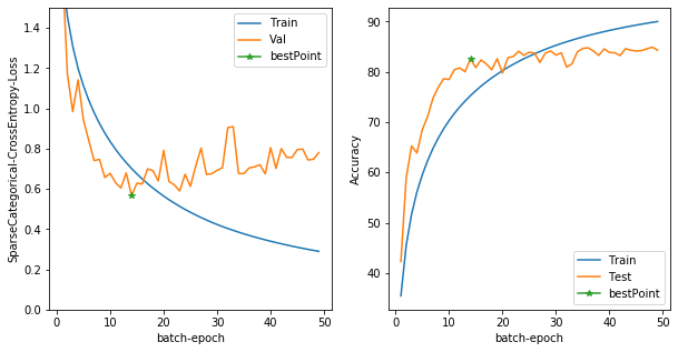
これで一旦学習させてみよう。
model = DNNmodel(name="DNNmodel")
train(model,"firstmodel")
100%|██████████| 40000/40000 [00:11<00:00, 3520.87it/s, Train_Loss: 1.75304, Train_Accuracy: 32.510]
the best mode!:loss1.99360,acc29.490
100%|██████████| 40000/40000 [00:09<00:00, 4031.21it/s, Train_Loss: 1.48647, Train_Accuracy: 44.206]
not best mode!:loss2.00988,acc41.300 stopcount:1
100%|██████████| 40000/40000 [00:09<00:00, 4000.77it/s, Train_Loss: 1.31734, Train_Accuracy: 51.237]
the best mode!:loss1.00378,acc64.390
...中略

not best mode!:loss0.79759,acc84.200 stopcount:32
100%|██████████| 40000/40000 [00:10<00:00, 3920.37it/s, Train_Loss: 0.29922, Train_Accuracy: 89.642]
not best mode!:loss0.74358,acc84.560 stopcount:33
100%|██████████| 40000/40000 [00:10<00:00, 3911.42it/s, Train_Loss: 0.29429, Train_Accuracy: 89.818]
not best mode!:loss0.74700,acc84.880 stopcount:34
100%|██████████| 40000/40000 [00:10<00:00, 3930.98it/s, Train_Loss: 0.28953, Train_Accuracy: 89.988]
not best mode!:loss0.78008,acc84.290 stopcount:35

the best score:

 Test Loss: 0.5882744193077087, Test Accuracy: 81.87999725341797
これをDataAugmentationで強化する。
どのようにDataAugmentationするかの方針はこちらのブログ、
データのお気持ちを考えながらData Augmentationする
を参考にさせていただきました。
また、どのように実装するかについてはこちらのブログ、
NumPyでの画像のData Augmentationまとめ
を参考にしました。
しかし、作成時間の関係で今回は簡単に実装できるものだけでDataAugmentationします...
後日また詳しいAugmentationについては紹介しようと思います。
(ここで詳しく語っても横道にそれてしまう感じがします)
(tf系でかつ高速なAugmentationをしようと思うと難しいのでひとまずはペンディングします)
@tf.function
def rotate_tf(image,label):
    if image.shape.__len__() ==4:

        random_angles = tf.random.uniform(shape = (tf.shape(image)[0], ), minval = -30*np
        .pi / 180, maxval = 30*np.pi / 180)
    if image.shape.__len__() ==3:
        random_angles = tf.random.uniform(shape = (), minval = -30*np
        .pi / 180, maxval = 30*np.pi / 180)

    return tfa.image.rotate(image,random_angles),label

@tf.function
def flip_left_right(image,label):
    return tf.image.random_flip_left_right(image),label

@tf.function
def flip_up_down(image,label):
    return tf.image.random_flip_up_down(image),label


(train_x, train_y), (test_x, test_y) =  keras.datasets.cifar10.load_data()
train_x, test_x = train_x/255.0, test_x/255.0
train_x,val_x,train_y,val_y = train_test_split(train_x,train_y,test_size=0.2,shuffle=True)
train_ds = tf.data.Dataset.from_tensor_slices((train_x,train_y)).shuffle(40000)
train_ds = train_ds.batch(128).map(flip_up_down).map(flip_left_right).map(rotate_tf)
val_ds = tf.data.Dataset.from_tensor_slices((val_x,val_y))
val_ds = val_ds.batch(128)
test_ds = tf.data.Dataset.from_tensor_slices((test_x,test_y))
test_ds = test_ds.batch(128)

model = DNNmodel(name="temp")
train(model,"temp")
...中略
100%|██████████| 40000/40000 [00:10<00:00, 3858.39it/s, Train_Loss: 0.50215, Train_Accuracy: 82.597]
not best mode!:loss0.46391,acc86.160 stopcount:27
100%|██████████| 40000/40000 [00:10<00:00, 3861.20it/s, Train_Loss: 0.50036, Train_Accuracy: 82.661]
not best mode!:loss0.44775,acc87.090 stopcount:28
100%|██████████| 40000/40000 [00:10<00:00, 3867.10it/s, Train_Loss: 0.49860, Train_Accuracy: 82.723]
not best mode!:loss0.41001,acc87.680 stopcount:29
100%|██████████| 40000/40000 [00:10<00:00, 3871.51it/s, Train_Loss: 0.49685, Train_Accuracy: 82.785]not best mode!:loss0.40719,acc87.510 stopcount:30
early stopping!!

the best score:

 Test Loss: 0.42540156841278076, Test Accuracy: 86.48999786376953
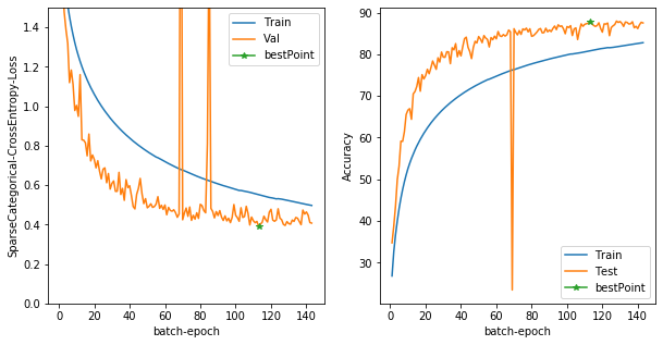
ちょっと途中でLossが爆発してるのが気になりますが...
すごくいい精度が出ました。ですが、90%を目指すならもっと工夫した方が良さそうですね。
次は、epochごとに学習率を変えてみることにしましょう。
学習率減衰
学習率を変える方法も簡単に変えられます。単純にoptimizerを学習途中で変えればいいのです。
def train(input_model,model_name="temp"):
    save_weight="/tmp/checkpoints/"+model_name

    train_loss = tf.keras.metrics.Mean(name='train_loss')
    train_accuracy = tf.keras.metrics.SparseCategoricalAccuracy(name='train_accuracy')
    #train_auc = tf.keras.metrics.AUC(name="train_auc")

    val_loss = tf.keras.metrics.Mean(name='val_loss')
    val_accuracy = tf.keras.metrics.SparseCategoricalAccuracy(name='val_accuracy')
    #val_auc = tf.keras.metrics.AUC(name="val_auc")

    test_loss = tf.keras.metrics.Mean(name='test_loss')
    test_accuracy = tf.keras.metrics.SparseCategoricalAccuracy(name='test_accuracy')
    #test_auc = tf.keras.metrics.AUC(name="test_auc")


    @tf.function
    def val_step(image, label):
        #testのoneStep
        predictions = input_model(image)
        t_loss = loss_object(label, predictions)

        val_loss(t_loss)
        val_accuracy(label, predictions)
        #val_auc.update_state(label, predictions)

    #max_auc=0.5
    min_loss =10000.0
    early_stop_count=0
    loss_object = tf.keras.losses.SparseCategoricalCrossentropy()
    stat_train_loss = []
    stat_train_acc = []
    #stat_train_auc = []
    stat_val_loss = []
    stat_val_acc = []
    #stat_val_auc = []
    stat_isbest = 0
    early_stop_limit = 30
    for epoch in range(1,250):
        if early_stop_count ==early_stop_limit and epoch >=50:
            print("early stopping!!")
            break

        if epoch <75:
            optimizer = tf.keras.optimizers.Adam(0.001)
        elif epoch >=75 and epoch <150 :
            optimizer = tf.keras.optimizers.Adam(0.0001)
        elif epoch >=150:
            optimizer = tf.keras.optimizers.Adam(0.00001)

        @tf.function
        def train_step(image, label):
            with tf.GradientTape() as tape:
                predictions = input_model(image,training=True)
                loss = loss_object(label,predictions)
            gradients = tape.gradient(loss, input_model.trainable_variables)
            optimizer.apply_gradients(zip(gradients, input_model.trainable_variables))

            train_loss(loss)
            train_accuracy(label, predictions)
            #train_auc.update_state(label, predictions)


        with tqdm(total=len(train_x))as pb:
            pb.set_description_str("Epoch:{}".format(epoch+1))
            for train_x_, train_y_ in train_ds:
                train_step(train_x_,train_y_)

                template = 'Train_Loss: {:.5f}, Train_Accuracy: {:.3f}'
                suffix=template.format(
                train_loss.result(),
                train_accuracy.result()*100,
                #train_auc.result(),
                )

                pb.set_postfix_str(suffix)
                pb.update(len(train_x_))
            stat_train_loss.append(train_loss.result())
            stat_train_acc.append(train_accuracy.result()*100)
            for val_x_,val_y_ in val_ds:
                val_step(val_x_,val_y_)
            if val_loss.result()<min_loss:
                input_model.save_weights(save_weight)
                min_loss = val_loss.result()
                stat_isbest+=early_stop_count+1
                early_stop_count = 0
                print("the best mode!:loss{:.5f},acc{:.3f}".format(val_loss.result(),val_accuracy.result()*100))
            else:
                print("not best mode!:loss{:.5f},acc{:.3f} stopcount:{}".format(val_loss.result(),val_accuracy.result()*100,early_stop_count+1))
                early_stop_count+=1

            stat_val_loss.append(val_loss.result())
            stat_val_acc.append(val_accuracy.result()*100)
            #stat_val_auc.append(val_auc.result())

            val_loss.reset_states()
            val_accuracy.reset_states()


    input_model.load_weights(save_weight)
    #test_auc = tf.keras.metrics.AUC(name="test_auc")
    @tf.function
    def test_step(image, label):
        #testのoneStep
        predictions = input_model(image)
        t_loss = loss_object(label, predictions)

        test_loss(t_loss)
        test_accuracy(label, predictions)
        #test_auc.update_state(label, predictions)

    for test_img, test_label in test_ds:
        test_step(test_img,test_label)
    print("the best score:")
    template = '\n Test Loss: {}, Test Accuracy: {}'# Test_AUC :{}'
    print(template.format(
        test_loss.result(),
        test_accuracy.result()*100,
        #test_auc.result()
        )
    )
    input_model.save_weights(save_weight+".acc{}".format(test_accuracy.result()*100))

    plt.figure(figsize=(10,5),facecolor="white")
    x_axis= list(range(1,len(stat_train_acc)+1))
    plt.subplot(121)
    plt.xlabel("batch-epoch")
    plt.ylabel("SparseCategorical-CrossEntropy-Loss")
    plt.ylim(0,1.5)
    plt.plot(x_axis,stat_train_loss)
    plt.plot(x_axis,stat_val_loss)
    plt.plot([stat_isbest],[stat_val_loss[stat_isbest-1]],marker="*")
    plt.legend(['Train', 'Val', 'bestPoint'], loc='upper right')

    plt.subplot(122)
    plt.xlabel("batch-epoch")
    plt.ylabel("Accuracy")
    plt.plot(x_axis,stat_train_acc)
    plt.plot(x_axis,stat_val_acc)
    plt.plot([stat_isbest],[stat_val_acc[stat_isbest-1]],marker="*")
    plt.legend(['Train', 'Test', 'bestPoint'], loc='lower right')

    """
    plt.subplot(133)
    plt.xlabel("batch-epoch")
    plt.ylabel("AUC")
    plt.plot(x_axis,stat_train_auc)
    plt.plot(x_axis,stat_val_auc,"r")
    plt.plot([stat_isbest],[stat_val_auc[stat_isbest]],marker="*")
    plt.suptitle(model_name)"""
    plt.show()
    print(stat_isbest)


model = DNNmodel(name="temp")
train(model,"temp")
not best mode!:loss0.40854,acc87.810 stopcount:28
Epoch:128: 100%|██████████| 40000/40000 [00:11<00:00, 3523.69it/s, Train_Loss: 0.53335, Train_Accuracy: 81.554]
not best mode!:loss0.40124,acc87.610 stopcount:29
Epoch:129: 100%|██████████| 40000/40000 [00:11<00:00, 3428.10it/s, Train_Loss: 0.53132, Train_Accuracy: 81.625]not best mode!:loss0.40338,acc87.740 stopcount:30
early stopping!!

the best score:

 Test Loss: 0.398386687040329, Test Accuracy: 87.97000122070312
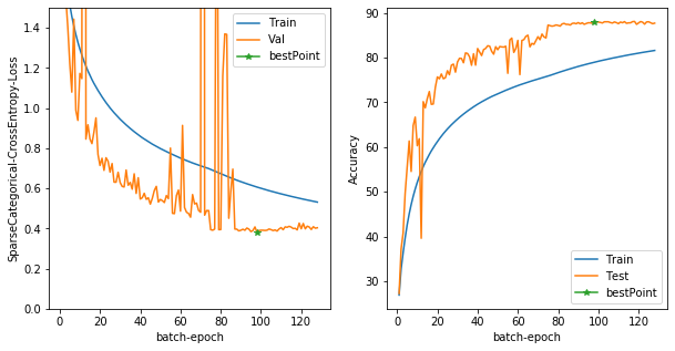
88%まで成長しましたね。
おわりに
こんな感じでいくらでもトレーニング中の動作を制御することができるようになりました。
tqdmを使えば進捗バーも出ますし、ハイレベルAPIと似た挙動をさせることも可能です。
このトレーニングループをベースにして、研究してみてください。
一旦、私の方でのAdventCalendarでのハンズオンはここまでになります。続きを書く時間があれば、空いているカレンダーに入れて、内容を投稿するかもしれません。
(Ganでのループとか、DataAugmentationとか)