続編記事
半加算器と全加算器をニューラルネットで作ってみる — 2次元の決定領域で学ぶ論理回路と MLP
導入
ニューラルネットワークは「重み付き和+活性化」という単純な仕組みで動く一方、層(深さ)と非線形を重ねるだけで表現できる関数の種類が飛躍的に増えます。本記事では、単一ニューロン=直線分離という事実から出発し、XOR が単層では解けないこと、そして2層(合計3ニューロン)で解けることを図と最小コードで確かめます。最後に、線形では分けられない同心円データで MLP の表現力を体感します。
1. 単一ニューロンで AND / OR / NAND
単一ニューロン(パーセプトロン)は y = step(w1*x1 + w2*x2 + b) で出力します。境界は直線 w·x + b = 0。以下は重みとバイアスの具体例と決定領域です。
- AND :
w=[1,1], b=-1.5 - OR :
w=[1,1], b=-0.5 - NAND:
w=[-1,-1], b=1.5
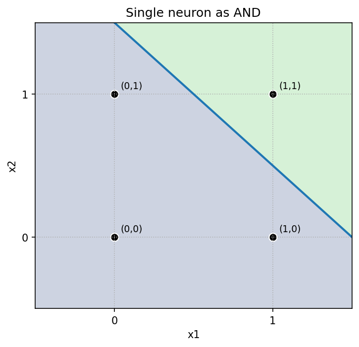
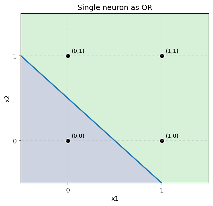
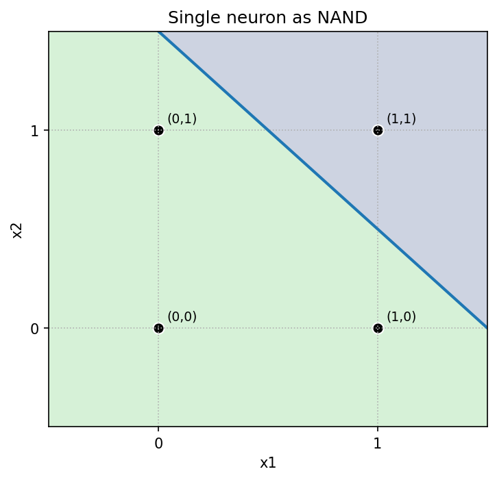
直感:バイアス(しきい値)を上げると判定が「厳しく」(AND)、下げると「緩く」(OR)なります。NAND は AND の符号反転です。
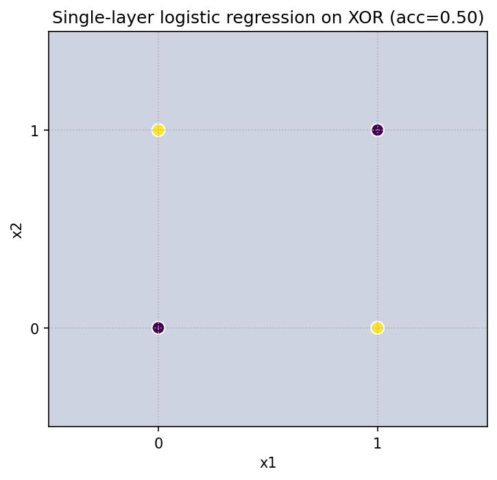
2. 単層では XOR を表現できない(線形分離不可)
XOR の真理値は (0,0)->0, (1,0)->1, (0,1)->1, (1,1)->0。
1 本の直線ではこの 4 点を分け切れません。線形モデル(ロジスティック回帰)で挑戦すると、必ず取りこぼしが生じます。
3. 2層3ニューロンなら XOR を「構成的」に実装できる
XOR は
XOR = OR AND NOT(AND)
と分解できます。隠れ層で OR と NANDを計算し、出力層で ANDをとれば完成です(合計 3 ニューロン)。
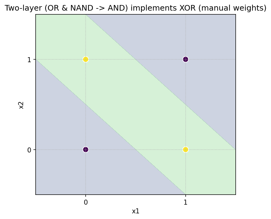
作れる(表現可能性)と学習で到達できる(最適化)は別問題。ここでは「作れる」ことを確認します。
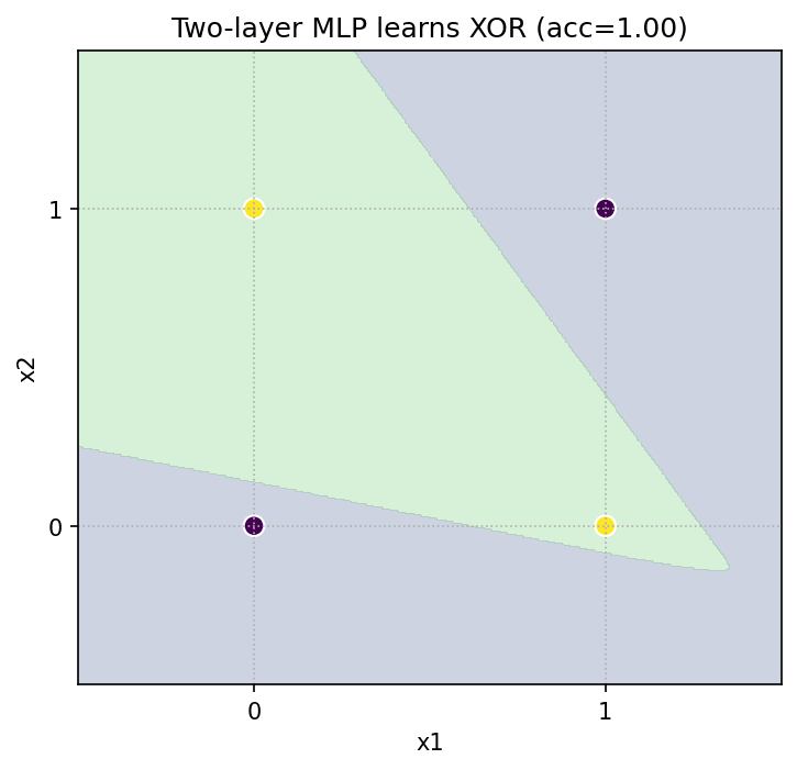
4. 学習でも確認:MLP は XOR を解ける
同じ 4 点のデータに対して、1 隠れ層の MLP を学習させると、正しく分離できる決定領域が得られます。
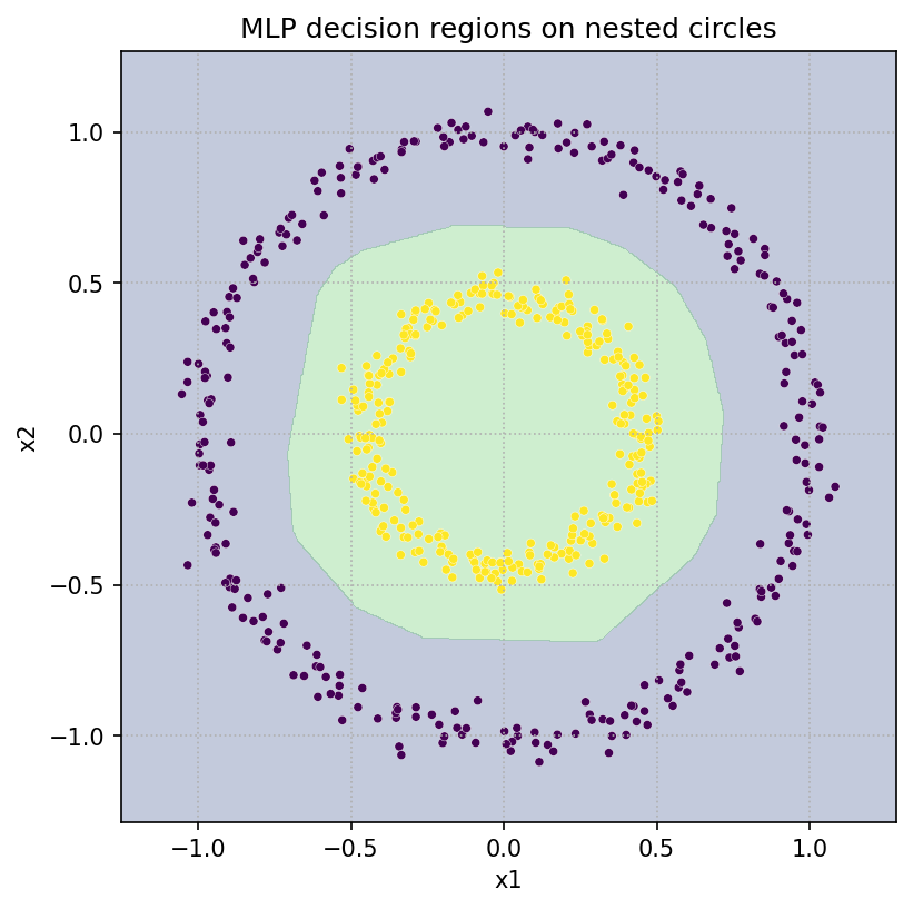
5. 多層 MLP の表現力:同心円データを分類
線形では絶対に分けられない同心円状のデータを、MLP が非線形の境界で分離します(make_circles、活性化 ReLU、隠れ 16-16)。
付録コード:1セルで記事中の図をすべて再現(保存つき)
# %pip -q install scikit-learn
import numpy as np, matplotlib.pyplot as plt, os
from itertools import product
from sklearn.linear_model import LogisticRegression
from sklearn.neural_network import MLPClassifier
from sklearn.datasets import make_circles

np.random.seed(0); os.makedirs("fig", exist_ok=True)

def step(z): return (z >= 0).astype(int)
def grid2d(xmin=-0.5, xmax=1.5, ymin=-0.5, ymax=1.5, n=400):
    xx, yy = np.meshgrid(np.linspace(xmin, xmax, n), np.linspace(ymin, ymax, n))
    X = np.stack([xx.ravel(), yy.ravel()], axis=1); return xx, yy, X

def plot_region_single_neuron(w, b, title, save):
    xx, yy, X = grid2d(); Z = step(X @ w + b).reshape(xx.shape)
    plt.figure(figsize=(6,6)); plt.contourf(xx, yy, Z, levels=[-0.5,0.5,1.5], alpha=0.25)
    if abs(w[1])>1e-6:
        xs = np.linspace(-0.5, 1.5, 200); ys = -(w[0]*xs + b)/w[1]; plt.plot(xs, ys, lw=2)
    else: plt.axvline(-b/w[0], lw=2)
    P = np.array(list(product([0,1],[0,1]))); plt.scatter(P[:,0], P[:,1], c='k', s=60, edgecolors='white')
    for a,bv in P: plt.text(a+0.04,bv+0.04,f"({a},{bv})",fontsize=9)
    plt.xlim(-0.5,1.5); plt.ylim(-0.5,1.5); plt.xticks([0,1]); plt.yticks([0,1])
    plt.title(title); plt.xlabel("x1"); plt.ylabel("x2"); plt.grid(True, ls=":")
    plt.savefig(save, dpi=150, bbox_inches='tight'); plt.show()

# Gates
w_and, b_and   = np.array([1.0,1.0]), -1.5
w_or,  b_or    = np.array([1.0,1.0]), -0.5
w_nand, b_nand = np.array([-1.0,-1.0]), 1.5
plot_region_single_neuron(w_and,  b_and,  "Single neuron as AND",  "fig/gate_and.png")
plot_region_single_neuron(w_or,   b_or,   "Single neuron as OR",   "fig/gate_or.png")
plot_region_single_neuron(w_nand, b_nand, "Single neuron as NAND", "fig/gate_nand.png")

# XOR: logistic regression fails (single-layer)
X = np.array([[0,0],[0,1],[1,0],[1,1]]); y = np.array([0,1,1,0])
logr = LogisticRegression(C=1e6, solver='lbfgs').fit(X, y)
xx, yy, gridX = grid2d(); Z_logr = logr.predict(gridX).reshape(xx.shape)
plt.figure(figsize=(6,6)); plt.contourf(xx, yy, Z_logr, levels=[-0.5,0.5,1.5], alpha=0.25)
plt.scatter(X[:,0], X[:,1], c=y, s=80, edgecolors='white')
plt.title(f"Single-layer logistic regression on XOR (acc={logr.score(X,y):.2f})")
plt.xlabel("x1"); plt.ylabel("x2"); plt.grid(True, ls=":"); plt.savefig("fig/xor_logreg.png", dpi=150, bbox_inches='tight'); plt.show()

# XOR: manual two-layer (OR & NAND -> AND)
h1 = step(gridX @ w_or + b_or); h2 = step(gridX @ w_nand + b_nand)
Z_manual = step(np.c_[h1,h2] @ np.array([1.0,1.0]) - 1.5).reshape(xx.shape)
plt.figure(figsize=(8,6)); plt.contourf(xx, yy, Z_manual, levels=[-0.5,0.5,1.5], alpha=0.25)
plt.scatter(X[:,0], X[:,1], c=y, s=80, edgecolors='white')
plt.title("Two-layer (OR & NAND -> AND) implements XOR (manual weights)")
plt.xlabel("x1"); plt.ylabel("x2"); plt.grid(True, ls=":"); plt.savefig("fig/xor_manual.png", dpi=150, bbox_inches='tight'); plt.show()

# XOR: learn with 2-layer MLP (hidden=2)
mlp_xor = MLPClassifier(hidden_layer_sizes=(2,), activation='logistic',
                        solver='lbfgs', alpha=1e-4, random_state=0, max_iter=10000).fit(X, y)
Z_mlp = mlp_xor.predict(gridX).reshape(xx.shape)
plt.figure(figsize=(6,6)); plt.contourf(xx, yy, Z_mlp, levels=[-0.5,0.5,1.5], alpha=0.25)
plt.scatter(X[:,0], X[:,1], c=y, s=80, edgecolors='white')
plt.title(f"Two-layer MLP learns XOR (acc={mlp_xor.score(X,y):.2f})")
plt.xlabel("x1"); plt.ylabel("x2"); plt.grid(True, ls=":"); plt.savefig("fig/xor_mlp.png", dpi=150, bbox_inches='tight'); plt.show()

# Expressivity: nested circles
from sklearn.datasets import make_circles
Xc, yc = make_circles(n_samples=600, noise=0.04, factor=0.45, random_state=0)
mlp_circles = MLPClassifier(hidden_layer_sizes=(16,16), activation='relu',
                            solver='adam', random_state=0, max_iter=4000).fit(Xc, yc)
xx2, yy2 = np.meshgrid(np.linspace(Xc[:,0].min()-0.2, Xc[:,0].max()+0.2, 600),
                       np.linspace(Xc[:,1].min()-0.2, Xc[:,1].max()+0.2, 600))
Zc = mlp_circles.predict(np.c_[xx2.ravel(), yy2.ravel()]).reshape(xx2.shape)
plt.figure(figsize=(7,7)); plt.contourf(xx2, yy2, Zc, levels=[-0.5,0.5,1.5], alpha=0.3)
plt.scatter(Xc[:,0], Xc[:,1], c=yc, s=15, edgecolors='white', linewidths=0.2)
plt.title("MLP decision regions on nested circles"); plt.xlabel("x1"); plt.ylabel("x2"); plt.grid(True, ls=":")
plt.savefig("fig/circles_mlp.png", dpi=150, bbox_inches='tight'); plt.show()