Link: https://arxiv.org/pdf/1506.00019.pdf
LaTex Command: https://qiita.com/PlanetMeron/items/63ac58898541cbe81ada#%E3%82%AE%E3%83%AA%E3%82%B7%E3%83%A3%E6%96%87%E5%AD%97
Abstract
Recurrent neural networks (RNNs) are connectionist models that capture the dynamics of sequences via cycles in the network of nodes. Unlike standard feedforward neural networks, recurrent networks retain a state that can represent information from an arbitrarily long context window.
In this survey, they review and summarise key researches of algorithms and its designs.
The goal is to provide an explanatory review with historical views.
- Introduction
- Why model sequentiality explicitly?
- Why not use Markov models?
- Are RNNs too expressive?
- Background
- Sequences
- Neural Networks
- Feedforward Networks and backpropagation
- RNN
- Early Recurrent Networks Designs
- Training Recurrent Networks
- Implementation
- Modern RNN
- LSTM (Long Short Term Memory)
- BRNNs (Bidirectional RNN)
- Neural Turing Machines
1. Introduction
Unlike traditional ML rely upon manual-engineered features, deep neural nets are suited well for machine perception tasks.
However, due to the explosively increase the amount of data, simple linear models tended to end up with under-fit of data. To tackle this issue, DNNs, which are aggressively built by evolutionary growth of certain architecture of DL. For instance, deep belief networks, boltzmann machine and CNN, have demonstrated ground-braking record in some tasks.
But none of these networks had the power to correctly represent the connection between past and present.
Hereby, RNN, which are connectionist models with the ability to selectively pass data across sequence steps while processing sequential data one element at a time, has been invented.
1.1 Why model sequentiality explicitly?
Advantages on conventional useful ML algorithms, like SVM and logistic regression.
- Easy to model with sequential data
- many models implicitly contain sequentiality inside by merging predecessors and successors of inputs
Disadvantages on Conventional models
Unable to include long-range dependencies!!
1.2 Why not use Markov models?
Frankly RNN is not the only models can represent time dependencies.
For instance, Markov chains, which model transitions between states in an observed sequence, and HMMs(Hidden Markov models) which model an observed sequence as probabilistically dependent upon a sequence of unobserved states.
However, if we extends the time steps hugely, it is infeasible for these markov models to calculate the transition probability using dynamic programming. Further, the basic concept of Markov is the present is independent of the history. hence not suited for largely sequential data.
Yet, hidden layers of RNN can maintain a nearly arbitrarily long context window.
1.3 Are RNNs too expressive?
First, given any fixed architecture (set of nodes, edges, and activation functions), the recurrent neural networks with this architecture are differentiable end to end. The derivative of the loss function can be calculated with respect to each of the parameters (weights) in the model. Thus, RNNs are amenable to gradient-based training.
Second, while the Turing-completeness of RNNs is an impressive property, given
a fixed-size RNN with a specific architecture, it is not actually possible to reproduce any arbitrary program.
1.4 Comparison to Prior literature
Other papers are garbage!!!
2. Background
2.1 Sequences
RNNs can be applied to not only time sequence, but also genetic data or any kind of sequential data
where T is called the maximum
input: (x^{(1)}, x^{(2)}, ..., x^{(T)})\\
output: (y^{(1)}, y^{(2)}, ..., y^{(T)})\\
2.2 Neural Networks (I skipped this part!)
v_j = l_j\biggl(\sum_{j'}w_{jj'}・v_{j'}\biggl)\\
\hat{y} = \frac{e^{a_k}}{\sum_{k'=1}^Ke^{a_{k'}}}
2.3 Feedforward Networks and backpropagation (I skipped this part!)
w \leftarrow w - \eta\nabla_wF_i\\
\delta_k = \frac{\partial L(\hat{y_k},y_k)}{\partial \hat{y_k}}・l_k'(a_k)\\
\delta_j = l'(a_j)\sum_k\delta_k・w_{kj}\\
\frac{\partial L}{\partial w_{jj'}} = \delta_j v_{j'}
3. Recurrent Neural Networks
h_{(t)} = \sigma(W^{hx}x^{(t)} + W^{(hh)}h^{(t-1)}+b_h)\\
\hat{y}^{(t)} = softmax(W^{(yh)}h^{(t)}+b_y)
where $W^{(hx)}$: weights matrix between inputs and hidden layers
$W^{(hh)}$: recurrent weights between hidden layer and itself, like looping
$b_h, b_y$: bias parameters
backpropagation through time: BPTT
image

3.1 Early Recurrent Network Designs
two architecture in RNN
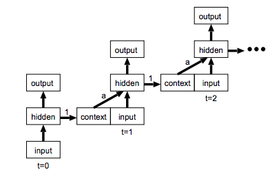
- Elman Model: Associate with each hidden units are contexts units. Good for NLP
reference: http://www.cis.twcu.ac.jp/~asakawa/chiba2002/lect4-SRN/recurrent-net.pdf
\begin{align}
h^{(t)}& = \sigma(I^{(t)} + ah^{(t-1)})\\
&= \sigma(I^{(t)} + a(I^{(t-1)} + h^{(t-2)}))\\
&= \sigma(I^{(t)} + aI^{(t-1)} + a^2h^{(t-2)} + a^2h^{(t-2)} ... a^nI^{(t-n)})\\
&= \sigma(\sum_{n=0}^T a^nI^{(t-n)})
\end{align}
- Jordan Model: good for robotics or some physical action
refence: https://www.researchgate.net/figure/Jordan-neural-network_fig1_266204519

3.2 Training Recurrent Networks
During the backpropagation of training step, we will face two fundamental issues related with Gradients
- Vanishing
- Exploding
For the simplicity, Let's consider a network with a single input node, a single output.

The transitions of weights over time steps indicates that the recurrent edge at the hidden node $j$ always has the same weight. Hence, the gradient of weights can be either explosive(suddenly spike from 0 to some point) or flatten(zero).
Therefore, the derivative of the error with respect to the input will either explode or vanish.
As for solution to these two issues, we have seen some smart methods.
- vanishing: use ReLu(Rectified Linear Unit max(0,x) ), instead of sigmoid
- exploding: add regularization term forcing the weights to values where the gradient neither vanishes nor explodes.
Training Step with Backpropagation through Time (BPTT)
Reference: http://ir.hit.edu.cn/~jguo/docs/notes/bptt.pdf
- dear Jiang Guo, I really appreciate your contribution by this paper!! you saved us!
At this point, Let's get our hands a bit dirty to obtain practical knowledge to update weights in RNN.
For the simplicity, I have pre-defined some of important variables below.
| variable | description | index |
|---|---|---|
| $x^t$ | input layer | i |
| $s^{t-1}$ | previous hidden layer | h |
| $s^{t}$ | current hidden layer | j |
| $y^t$ | output layer | k |
| $W$ | current hidden layer $\rightarrow$ output | j, k |
| $V$ | input layer $\rightarrow$ current hidden layer | i, j |
| $V$ | previous hidden layer $\rightarrow$ current hidden layer | h, j |
Procedure
Forwardpropagation
Input $\rightarrow$ Hidden layer
- Activate Neurons
- Forward Propagation
Hidden layer $\rightarrow$ Output layer
- Activate Neurons
- Forward Propagation
Define Cost Function
Backpropagation using BPTT to update each weight matrix ($W$,$V$,$U$)
- Hidden layer $\leftarrow$ Output layer
- Input $\leftarrow$ Hidden layer
Image of the architecture of the network

Calculation
Forwardpropagation
Input $\rightarrow$ Hidden layer
- Activate Neurons ($f$ is an activate function, like sigmoid)
s^t = f(net^t_j)
- Forward Propagation
net^t_j = \sum^I_i V^T_{ij} x_i + \sum^m_h U^T_{hj} s^{t-1}_h + b_j
Hence current Hidden layer looks like
s^t = f\bigl( \sum^I_i V^T_{ij} x_i + \sum^m_h U^T_{hj} s^{t-1}_h + b_j \bigl)
Hidden layer $\rightarrow$ Output layer
- Activate Neurons
y^t_k = g(net^t_k)
- Forward Propagation
net^t_k = \sum^m_j W^T_{jk} s^t_j + b_k
Hence output layer looks like
y^t_k = g\bigl( \sum^m_j W^T_{jk} s^t_j + b_k \bigl)\\
y^t_k = g\biggl( \sum^m_j W^T_{jk} \bigl(f\bigl( \sum^I_i V^T_{ij} x_i + \sum^m_h U^T_{hj} s^{t-1}_h + b_j \bigl) \bigl) + b_k \biggl)
Define Cost Function
- SSE(Summed Squared Error): $ C = \frac{1}{2}\sum^n_p \sum^o_k (d_{pk} - y_{pk})^2 $
- Cross Entropy: $ C = -\sum^n_p \sum^o_k \bigl(d_{pk} \ln y_{pk} + (1 - d_{pk}) \ln (1 - y_{pk}) \bigl) $
Backpropagation using BPTT
- Hidden layer $\leftarrow$ Output layer
\Delta w = - \eta \frac{\partial C}{\partial w} = - \eta \overbrace{\frac{\partial C}{\partial net_{pk}}}^{Non Linear} \overbrace{\frac{\partial net_{pk}}{\partial w}}^{Linear} \rightarrow
\left\{
\begin{array}{ll}
- \frac{\partial C}{\partial net_{pk}} = - \frac{\partial C}{\partial y_{pk}} \frac{\partial y_{pk}}{\partial net_{pk}} = (d_{pk} - y_{pk})g'(net_{pk}) = \delta_{pk}\\
\frac{\partial net_{pk}}{\partial w} = s^t_j
\end{array}
\right.\\

\Delta w_{kj} = \eta \sum^n_p \delta_{pk} s^t_{pj}
- Input $\leftarrow$ Hidden layer
\Delta v = - \eta \frac{\partial C}{\partial v} = -\eta \frac{\partial C}{\partial net_{pk}} \frac{\partial net_{pk}}{\partial s^t} \frac{\partial s^t}{\partial net_{pj}} \frac{\partial net_{pj}}{\partial v} \\

\Delta v_{ji} = -\eta \sum^n_p \delta_{pk} w_{kj} f'(net_{pj}) x_{pi} \\
Likewise \\
\Delta u_{ji} = -\eta \sum^n_p \delta_{pk} w_{kj} f'(net_{pj}) s^{t-1}_{pi} \\
*Truncated Backpropagation Algorithm is well described here
Ilya Sutskever, Training Recurrent Neural Networks, Thesis, 2013
*nice summary
https://machinelearningmastery.com/gentle-introduction-backpropagation-time/
Summary of the Vanishing Gradients problem
Understanding The Difficulty of Training Deep Feedforward Neural Network
https://qiita.com/Rowing0914/items/372e403bf1eda65f8c15
Implementation
Followed this blog!
http://www.wildml.com/2015/09/recurrent-neural-networks-tutorial-part-2-implementing-a-language-model-rnn-with-python-numpy-and-theano/
This code is uploaded on Github
https://github.com/Rowing0914/NeuralNetwork_DeepLearning/blob/master/src/nn_scratch_denny/nn_from_scratch.py
import numpy as np
import csv
import itertools
import operator
import nltk
import sys
from datetime import datetime
from utils import *
import matplotlib.pyplot as plt
class RNNNumpy:
def __init__(self, word_dim, nepoch, learning_rate, gradient_check_threshold, hidden_dim, bptt_truncate):
# Assign instance variables
self.word_dim = word_dim
self.hidden_dim = hidden_dim
self.bptt_truncate = bptt_truncate
self.learning_rate = learning_rate
self.nepoch = nepoch
self.h = 0.01
self.error_threshold = gradient_check_threshold
# Randomly initialize the network parameters
self.W = np.random.uniform(-np.sqrt(1./word_dim), np.sqrt(1./word_dim), (hidden_dim, word_dim))
self.V = np.random.uniform(-np.sqrt(1./hidden_dim), np.sqrt(1./hidden_dim), (word_dim, hidden_dim))
self.U = np.random.uniform(-np.sqrt(1./hidden_dim), np.sqrt(1./hidden_dim), (hidden_dim, hidden_dim))
def forward_propagation(self, x):
# The total number of time steps
T = len(x)
# During forward propagation we save all hidden states in s because need them later.
# We add one additional element for the initial hidden, which we set to 0
s = np.zeros((T + 1, self.hidden_dim))
s[-1] = np.zeros(self.hidden_dim)
# The outputs at each time step. Again, we save them for later.
o = np.zeros((T, self.word_dim))
# For each time step...
for t in np.arange(T):
# Note that we are indxing U by x[t]. This is the same as multiplying U with a one-hot vector.
s[t] = np.tanh(self.W[:,x[t]] + self.U.dot(s[t-1]))
o[t] = softmax(self.V.dot(s[t]))
return [o, s]
def predict(self, x):
# Perform forward propagation and return index of the highest score
o, s = self.forward_propagation(x)
return np.argmax(o, axis=1)
def calculate_total_loss(self, x, y):
L = 0
# For each sentence...
for i in np.arange(len(y)):
o, s = self.forward_propagation(x[i])
# We only care about our prediction of the "target" words
correct_word_predictions = o[np.arange(len(y[i])), y[i]]
"""
We could access of targe word's vector in that sentence
So (np.arange(len(y[i])), y[i]), this equates (array[0,1,2,...,length_of_sentence-1], index_word)
=====Accessing to the list elements by list of index=====
np.random.seed(0)
a = np.random.randn(10,20)
Idx = np.arange(3)
print a[Idx,1]
#output
[ 0.40015721 0.6536186 -1.42001794]
"""
# Add to the loss based on how off we were
L += -1 * np.sum(np.log(correct_word_predictions))
"""
=====elaboration of cross entropy=====
y = np.array([[0],[1],[0],[0]])
o = np.array([[0.3],[0.2],[0.15],[0.35]])
print "y * np.log(o)"
print y * np.log(o)
print "np.log(np.dot(o.T,y))"
print np.log(np.dot(o.T,y))
print np.sum(y * np.log(o)) ,np.sum(np.log(np.dot(o.T,y)))
# output
y * np.log(o)
[[-0. ]
[-1.60943791]
[-0. ]
[-0. ]]
np.log(np.dot(o.T,y))
[[-1.60943791]]
-1.60943791243 -1.60943791243
=====exponential of decimal numbers will be negative=====
print np.log(0.00012523)
# output
-8.98535851139
"""
return L
def calculate_loss(self, x, y):
# Divide the total loss by the number of training examples
N = np.sum((len(y_i) for y_i in y))
return self.calculate_total_loss(x,y)/N
def from_index_to_word(index_words):
res = []
for i in index_words:
res.append(index_to_word[i])
return res
# you can check his blog post as well
# http://www.wildml.com/2015/10/recurrent-neural-networks-tutorial-part-3-backpropagation-through-time-and-vanishing-gradients/
def bptt(self, x, y):
T = len(y)
# Perform forward propagation
o, s = self.forward_propagation(x)
# We accumulate the gradients in these variables
dLdU = np.zeros(self.W.shape)
dLdV = np.zeros(self.V.shape)
dLdW = np.zeros(self.U.shape)
delta_o = o
# calculate the error of prediction : (target - predict), namely, (1 - outcome of softmax)
delta_o[np.arange(len(y)), y] -= 1.
"""
=====sample code=====
o = np.array([ 0.00012408, 0.0001244, 0.00012603, 0.00012515, 0.00012488])
o -= 1.
print o
# output
[-0.99987592 -0.9998756 -0.99987397 -0.99987485 -0.99987512]
"""
# For each output backwards...
for t in np.arange(T)[::-1]:
"""
=====slice & reverse of list => LIST[::-1]=====
Link: https://stackoverflow.com/questions/3705670/best-way-to-create-a-reversed-list-in-python
LIST[::-1] <= this smart guy slices the whole sequence, with a step of -1, i.e., in reverse
a = "Hello World!!"
print a[::-1]
# output
!!dlroW olleH
"""
# error * activated hidden layer
dLdV += np.outer(delta_o[t], s[t].T)
"""
short summary : What we do here is obtaining the weight matrix for updating V
detali of components :
o : softmax( Vs + b )
delta_o : error signal(check the code above!!)
s : activated hidden layer, which is the input of softmax =>
V : weight matrix for output layer
b : bias
Example of calculation:
delta_o = [error_1 , error_2, error_3, .... ]
s = [s_1, s_2, s_3, .... ]
the outer product of these two will be below
outcome = [[error_1*s_1, error_1*s_2, error_1*s_3, .... ],
[error_2*s_1, error_2*s_2, error_2*s_3, .... ],
[error_3*s_1, error_3*s_2, error_3*s_3, .... ],
....
....
....
]
In conclusion, with outer product, we could update the weight matrix
As for outer product in numpy, check this link:
https://deepage.net/features/numpy-outer.html
https://en.wikipedia.org/wiki/Outer_product
=====np.outer=====
a = np.linspace(-2, 2, 5)
b = np.linspace(12, 52, 5)
print a.reshape(-1,1)*b
print np.outer(a,b)
print np.outer(a,b.T)
# output : same matrices!!
[[ -24. -44. -64. -84. -104.]
[ -12. -22. -32. -42. -52.]
[ 0. 0. 0. 0. 0.]
[ 12. 22. 32. 42. 52.]
[ 24. 44. 64. 84. 104.]]
[[ -24. -44. -64. -84. -104.]
[ -12. -22. -32. -42. -52.]
[ 0. 0. 0. 0. 0.]
[ 12. 22. 32. 42. 52.]
[ 24. 44. 64. 84. 104.]]
[[ -24. -44. -64. -84. -104.]
[ -12. -22. -32. -42. -52.]
[ 0. 0. 0. 0. 0.]
[ 12. 22. 32. 42. 52.]
[ 24. 44. 64. 84. 104.]]
"""
# Initial delta calculation
"""
tanh's derivativation is (1 - tanh(x)^2)
delta_t = V.T dot error * (1 - tanh(x)^2)
"""
delta_t = self.V.T.dot(delta_o[t]) * (1 - (s[t] ** 2))
# Backpropagation through time (for at most self.bptt_truncate steps)
for bptt_step in np.arange(max(0, t-self.bptt_truncate), t+1)[::-1]:
# print "Backpropagation step t=%d bptt step=%d " % (t, bptt_step)
"""
dLdW += (V.T dot error * (1 - tanh(x)^2)) dot previous_hidden
dLdU[:,x[bptt_step]] += (V.T dot error * (1 - tanh(x)^2)) dot previous_input??
"""
dLdW += np.outer(delta_t, s[bptt_step-1].T)
dLdU[:,x[bptt_step]] += delta_t
# Update delta for next step
# one time step backprop
delta_t = self.U.T.dot(delta_t) * (1 - s[bptt_step-1] ** 2)
return [dLdU, dLdV, dLdW]
def gradient_check(self, x, y):
# Calculate the gradients using backpropagation. We want to checker if these are correct.
bptt_gradients = model.bptt(x, y)
# List of all parameters we want to check.
model_parameters = ['U', 'V', 'W']
# Gradient check for each parameter
for pidx, pname in enumerate(model_parameters):
# Get the actual parameter value from the mode, e.g. model.W
parameter = operator.attrgetter(pname)(self)
"""
Above code tries to access the member attributes(U, V, W) of RNNNumpy class one by one.
Check this link!: https://docs.python.org/2/library/operator.html#operator.attrgetter
"""
print "Performing gradient check for parameter %s with size %d." % (pname, np.prod(parameter.shape))
# Iterate over each element of the parameter matrix, e.g. (0,0), (0,1), ...
it = np.nditer(parameter, flags=['multi_index'], op_flags=['readwrite'])
"""
=====np.nditer=====
we can access to each element by above one liner!
# code
np_array = np.random.randn(2, 3)
print "np_array","\n", np_array
nditer = np.nditer(np_array, flags=['multi_index'])
while not nditer.finished:
print nditer.multi_index
print np_array[nditer.multi_index]
nditer.iternext()
#output
np_array
[[-0.94897844 -0.1013277 -0.94604283]
[-1.05055428 -1.00631297 -2.38182881]]
(0, 0)
-0.948978439054
(0, 1)
-0.101327697174
(0, 2)
-0.94604283326
(1, 0)
-1.05055428018
(1, 1)
-1.00631296902
(1, 2)
-2.38182880702
"""
while not it.finished:
ix = it.multi_index
# Save the original value so we can reset it later
original_value = parameter[ix]
# Estimate the gradient using (f(x+h) - f(x-h))/(2*h)
"""
parameter[ix] is now accessing to the member attributes of RNNNumpy.
So (parameter[ix] = original_value + h) and (parameter[ix] = original_value - h) are affecting self.some_weight directly!!
That's why we need model.calculate_total_loss([x],[y]) twice!
"""
parameter[ix] = original_value + self.h
gradplus = model.calculate_total_loss([x],[y])
parameter[ix] = original_value - self.h
gradminus = model.calculate_total_loss([x],[y])
estimated_gradient = (gradplus - gradminus)/(2*self.h)
# Reset parameter to original value
parameter[ix] = original_value
# The gradient for this parameter calculated using backpropagation
backprop_gradient = bptt_gradients[pidx][ix]
# calculate The relative error: (|a - b|/(|a| + |b|))
# http://mathworld.wolfram.com/RelativeError.html
"""
As 'a' gets closer to 'b', the relative error decrease.
=====relative error=====
a = np.array([000000.1, 0.5, 0.79, 1000])
b = 0.8
print np.abs(a-b)/np.abs(a+b)
#output
[ 0.77777778 0.23076923 0.00628931 0.99840128]
"""
relative_error = np.abs(backprop_gradient - estimated_gradient)/(np.abs(backprop_gradient) + np.abs(estimated_gradient))
# If the error is to large fail the gradient check
if relative_error > self.error_threshold:
print "Gradient Check ERROR: parameter=%s ix=%s" % (pname, ix)
print "+h Loss: %f" % gradplus
print "-h Loss: %f" % gradminus
print "Estimated_gradient: %f" % estimated_gradient
print "Backpropagation gradient: %f" % backprop_gradient
print "Relative Error: %f" % relative_error
return
it.iternext()
print "Gradient check for parameter %s passed." % (pname)
# Performs one step of SGD.
def numpy_sdg_step(self, x, y):
# Calculate the gradients
dLdU, dLdV, dLdW = self.bptt(x, y)
# Change parameters according to gradients and learning rate
self.W -= self.learning_rate * dLdU
self.V -= self.learning_rate * dLdV
self.U -= self.learning_rate * dLdW
# Outer SGD Loop
# - model: The RNN model instance
# - X_train: The training data set
# - y_train: The training data labels
# - learning_rate: Initial learning rate for SGD
# - nepoch: Number of times to iterate through the complete dataset
# - evaluate_loss_after: Evaluate the loss after this many epochs
def train_with_sgd(self, model, X_train, y_train, evaluate_loss_after=5):
# We keep track of the losses so we can plot them later
losses = []
num_examples_seen = 0
for epoch in range(self.nepoch):
# Optionally evaluate the loss
if (epoch % evaluate_loss_after == 0):
loss = model.calculate_loss(X_train, y_train)
losses.append((num_examples_seen, loss))
time = datetime.now().strftime('%Y-%m-%d %H:%M:%S')
print "%s: Loss after num_examples_seen=%d epoch=%d: %f" % (time, num_examples_seen, epoch, loss)
# Adjust the learning rate if loss increases
if (len(losses) > 1 and losses[-1][1] > losses[-2][1]):
self.learning_rate = self.learning_rate * 0.5
print "Setting learning rate to %f" % self.learning_rate
sys.stdout.flush()
# For each training example...
for i in range(len(y_train)):
# One SGD step
model.sgd_step(X_train[i], y_train[i], self.learning_rate)
num_examples_seen += 1
# not working .....
def mini_batch_train_with_sgd(self, model, X_train, y_train, mini_batch_size=100, learning_rate=0.005, nepoch=100, evaluate_loss_after=5):
# We keep track of the losses so we can plot them later
losses = []
num_examples_seen = 0
for epoch in range(nepoch):
# create mini-batch training dataset.
mini_batches = np.arange(0, len(X_train), mini_batch_size)
"""
[i for i in range(0, 100, 20)] => [0, 20, 40, 60, 80]
this means the index of mini-batch
"""
for mini_batch in mini_batches:
loss = model.calculate_loss(X_train[mini_batch:mini_batch+mini_batch_size], y_train[mini_batch:mini_batch+mini_batch_size])
losses.append((num_examples_seen, loss))
time = datetime.now().strftime('%Y-%m-%d %H:%M:%S')
print "%s: Loss after num_examples_seen=%d epoch=%d: loss=%f" % (time, num_examples_seen, epoch, loss)
# Adjust the learning rate if loss increases
if (len(losses) > 1 and losses[-1][1] > losses[-2][1]):
learning_rate = learning_rate * 0.5
print "Setting learning rate to %f" % learning_rate
sys.stdout.flush()
# For each training example...
for mini_batch in mini_batches:
# One SGD step
model.sgd_step(X_train[mini_batch:mini_batch+mini_batch_size], y_train[mini_batch:mini_batch+mini_batch_size], learning_rate)
num_examples_seen += 1
def generate_sentence(model):
# We start the sentence with the start token
new_sentence = [word_to_index[sentence_start_token]]
# Repeat until we get an end token
while not new_sentence[-1] == word_to_index[sentence_end_token]:
next_word_probs, _ = model.forward_propagation(new_sentence)
sampled_word = word_to_index[unknown_token]
# We don't want to sample unknown words
while sampled_word == word_to_index[unknown_token]:
samples = np.random.multinomial(1, next_word_probs[-1])
"""
format: numpy.random.multinomial(n, pvals, size=None)
description: draw samples following the pvals distribution.
Link: https://docs.scipy.org/doc/numpy/reference/generated/numpy.random.multinomial.html
Link: https://stackoverflow.com/questions/29014620/use-np-random-multinomial-in-python
=====sampling methods=====
print np.random.multinomial(20, [1/6.]*6)
print sum(np.random.multinomial(20, [1/6.]*6))
a = softmax(np.random.randn(10))
print a
print np.random.multinomial(100, a, 1 )
print sum(np.random.multinomial(100, a, 1))
#output
[5 4 1 3 2 5]
20
[ 0.0651358 0.08968716 0.07765962 0.36091358 0.09490753 0.08519846
0.06437316 0.03076936 0.0554286 0.07592674]
[[ 9 11 7 36 4 8 12 3 2 8]]
[ 7 15 12 36 8 6 5 3 4 4]
"""
sampled_word = np.argmax(samples)
new_sentence.append(sampled_word)
sentence_str = [index_to_word[x] for x in new_sentence[1:-1]]
return sentence_str
class DataPreparation():
def __init__(self, word_dim, sentence_start_token, sentence_end_token):
self.word_dim=word_dim
self.sentence_start_token=sentence_start_token
self.sentence_end_token=sentence_end_token
def data_preprocessing(self):
# Read the data and append SENTENCE_START and SENTENCE_END tokens
print "Reading CSV file..."
with open('data/reddit-comments-2015-08.csv', 'rb') as f:
reader = csv.reader(f, skipinitialspace=True)
reader.next()
# Split full comments into sentences
sentences = itertools.chain(*[nltk.sent_tokenize(x[0].decode('utf-8').lower()) for x in reader])
# Append SENTENCE_START and SENTENCE_END
sentences = ["%s %s %s" % (self.sentence_start_token, x, self.sentence_end_token) for x in sentences]
print "Parsed %d sentences." % (len(sentences))
# Tokenize the sentences into words
tokenized_sentences = [nltk.word_tokenize(sent) for sent in sentences]
# Count the word frequencies
word_freq = nltk.FreqDist(itertools.chain(*tokenized_sentences))
print "Found %d unique words tokens." % len(word_freq.items())
# Get the most common words and build index_to_word and word_to_index vectors
vocab = word_freq.most_common(word_dim-1)
index_to_word = [x[0] for x in vocab]
index_to_word.append(unknown_token)
word_to_index = dict([(w,i) for i,w in enumerate(index_to_word)])
print "Using vocabulary size %d." % word_dim
print "The least frequent word in our vocabulary is '%s' and appeared %d times." % (vocab[-1][0], vocab[-1][1])
# Replace all words not in our vocabulary with the unknown token
for i, sent in enumerate(tokenized_sentences):
tokenized_sentences[i] = [w if w in word_to_index else unknown_token for w in sent]
print "\nExample sentence: '%s'" % sentences[0]
print "\nExample sentence after Pre-processing: '%s'" % tokenized_sentences[0]
# Create the training data
X_train = np.asarray([[word_to_index[w] for w in sent[:-1]] for sent in tokenized_sentences])
y_train = np.asarray([[word_to_index[w] for w in sent[1:]] for sent in tokenized_sentences])
return X_train, y_train
if __name__ == '__main__':
word_dim = 8000
learning_rate = 0.005
nepoch = 100
hidden_dim=100
bptt_truncate=4
gradient_check_threshold = 0.001
unknown_token = "UNKNOWN_TOKEN"
sentence_start_token = "SENTENCE_START"
sentence_end_token = "SENTENCE_END"
np.random.seed(10)
data = DataPreparation(word_dim, sentence_start_token, sentence_end_token)
X_train, y_train = data.data_preprocessing()
# Train on a small subset of the data to see what happens
print "Initialise Model"
model = RNNNumpy(word_dim, nepoch, learning_rate, gradient_check_threshold, hidden_dim, bptt_truncate)
print "Train Model"
model.train_with_sgd(model, X_train, y_train, evaluate_loss_after=1)
print "Training done!"
print "Generate random sentence based on the model!"
print "Let's see how it goes!"
num_sentences = 10
senten_min_length = 7
for i in range(num_sentences):
sent = []
# We want long sentences, not sentences with one or two words
while len(sent) < senten_min_length:
sent = generate_sentence(model)
print " ".join(sent)
4. Modern Architecture of RNNs
4.1 LSTM(Long Short Term Memory)
Check this my note out!!
https://qiita.com/Rowing0914/items/1edf16ead2190308ce90