[Review] Long Short Term Memory in 1997 #DeepLearning

1997 version ~Discovery of CEC~

Link

http://www.bioinf.jku.at/publications/older/2604.pdf
1999 version : https://qiita.com/Rowing0914/items/cefa095c761e11dcc3ad

Implementation

Author

Sepp Hochreiter
Jurgen Schmidhuber

Agenda

Introduction
Previous Work
Constant Error Backprop
1. Exponentially Decaying Error
2. Constant Error Flow: Naive Approach
Long Short Term Memory
Experiments
1. Experiment 1: Embedded Reber Grammar
2. Experiment 2: Noise-free and Noisy Sequences
3. Experiment 3: Noise and Signal on Same channel
4. Experiment 4: Adding Problem
5. Experiment 5: Multiplication Problem
6. Experiment 6: Temporal Order
7. Summary of Experimental Conditions
Discussion

1. Abstruct&Introduction

LSTM was invented to overcome the issue which learning to store information over extended time intervals takes very long time.
And it does learn to bridge minimal time lags in excess of 1000 discrete time steps.s by enforcing constant error flow through "constant error carrousels" within special units. Multiplicative units learn to open and close its gate.
Finally, LSTM is able to lean fastest among other algorithms, like BPTT, RTRL, RCC, Elman-Nets, neural sequence chunking.

The problem
while BPTT/RTRL propagating error signals through layers, it either blows up or vanishes. those lead us to end up with oscillating weights or takes prohibitive amount of time to train.
The remedy
LSTM can lean to bridge time intervals in excess of 1000 steps even in case of noisy. And this is achieved by an efficient gradient algorithm for an architecture enforcing constant error flow through internal states of special units.

2. Previous Work

Brief review of previous work.

Gradient-descent variant
those approaches suffer from the same problems as BPTT/RTRL. *couldn't find any material any more.

Time-Delays
updating unit activations based on a weighted sum of old activations *

Time-constants
using time constants influencing changes of unit activations, but for long term, time constant requires fine tuning and mostly impractical...

Ring's approach
adding higher units to network whenever it receives conflicting error signals. this is not applicable for unseen data.

Bengio et al's approaches

Bengio et al. (1994) investigate methods such as simulated annealing, multi-grid random search, time-weighted pseudo-Newton optimization, and discrete error propagation. Their \latch" and \2-sequence" problems are very similar to problem 3a with minimal time lag 100 (see Experiment 3). Bengio and Frasconi (1994) also propose an EM approach for propagating targets. With n so-called \state networks", at a given time, their system can be in one of only n dierent states. See also beginning of Section 5. But to solve continuous problems such as the \adding problem" (Section 5.4), their system would require an unacceptable number of states (i.e., state networks).

Kalman Filters
using kalman filter. Since they use \a derivative discount factor imposed to decay exponentially the effects of past dynamic derivatives," there is no reason to believe that their methods work.

Second order nets

(1) Watrous and Kuhn's architecture does not enforce constant error ow and is not designed to solve long time lag problems. (2) It has fully connected second-order sigma-pi units, while the LSTM architecture's MUs are used only to gate access to constant error ow. (3) Watrous and Kuhn's algorithm costs $O(W^2)$ operations per time step, ours only O(W), where W is the number
of weights.

Simple weight guessing
to avoid long term lag problems, they simply initialise the weights of layers with random numbers. sometime works well, but this can be impractical because its guess is not appropriate for huge amount of parameters or high weight precision.

Adaptive sequence chunkers

Schmidhuber's hierarchical chunker systems (1992b, 1993) do have a capability to bridge arbitrary time lags, but only if there is local predictability across the subsequences causing the time lags

3. CONSTANT ERROR BACKPROP

3.1 EXPONENTIALLY DECAYING ERROR

Summary about the vanishing error by backpropagating through layers(long time dependencies).

3.2 CONSTANT ERROR FLOW: NAIVE

Constant Error Carousel was introduced in this section.

Basic concept

4. LONG SHORT-TERM MEMORY

Image

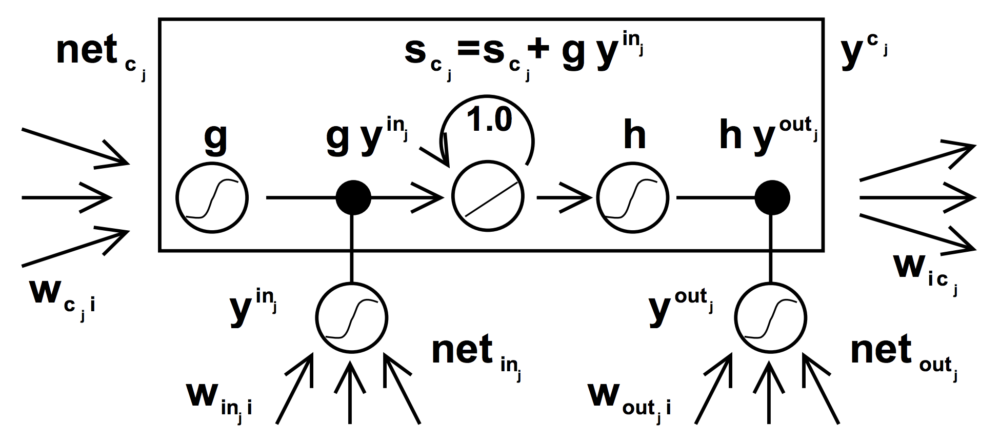
Forward Propagation

f(x) = \frac{1}{1+e^{-x}}\\
h(x) = \frac{2}{1+e^{-x}} - 1\\
g(x) = \frac{4}{1+e^{-x}} - 2\\

Before checking math, ensure that the input $y^u(t-1)$ equates the hidden calculation in conventional RNN. Hence it looks like this.
$y^u(t-1) = Wx_t + Uh_{t−1}$

The net input and the activation of hidden unit $i$

net_i(t) = \sum w_{iu} y^u(t-1)\\
y^i(t) = f_i(net_i(t))

$j$ th unit of memory cell unit $C$

net_{C^v_j}(t) = \sum_u w^v_{C^v_ju} y^u(t-1)\\
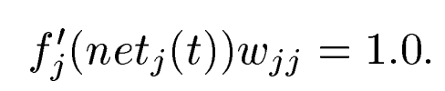
S_{C^v_j}(t) = 1(CEC \space coefficient) * S_{C^v_j}(t-1) + y^{in_j}(t)g(net_{C^v_j}(t))\\
y^{C^v_j}(t) = y^{out_j}(t)h(S_{C^v_j}(t))

The net input and the activation of $in_j$

net_{in_j}(t) = \sum w_{in_j u} y^u(t-1)\\
y^{in_j}(t) = f_{in_j}(net_{in_j}(t))

The net input and the activation of $out_j$

net_{out_j}(t) = \sum w_{out_j u} y^u(t-1)\\
y^{out_j}(t) = f_{out_j}(net_{out_j}(t))

The net input and the activation of output $k$

net_k(t) = \sum w_{k u} y^u(t-1)\\
y^{k}(t) = f_{k}(net_{k}(t))

Backpropagation

Firstly, let us define the cost function, which is using Squared error.
$E(t) = \sum_k (T^k(t) - y^k(t))^2$
where T means target, and y indicates output of LSTM

Procedure for BackProp

Explanation on Truncated BPTT
Complete Backprop Equation
Breaking equation down into components
SGD update for each weight matrix
Internal state updating

1. Explanation on Truncated BPTT

To ensure non-decaying error backprop through internal states of memory cells, we are going to truncate some part of backprop.
In this paper, they truncate "net input for memory cells", for instance $net_{c_j}, net_{in_j}, net_{out_j}$ meaning net inputs of in/output gates and cell itself. So Only within memory cells, errors are propagated back through
previous internal states $S_{C_j}$ .

\frac{\partial net_{in_j}(t)}{\partial y^u(t-1)} \approx_{tr} 0 \space forall \space u\\
\frac{\partial net_{out_j}(t)}{\partial y^u(t-1)} \approx_{tr} 0 \space forall \space u\\
\frac{\partial net_{C_j}(t)}{\partial y^u(t-1)} \approx_{tr} 0 \space forall \space u\\
Therefore \space we \space get\\
\frac{\partial y^{in_j}(t)}{\partial y^u(t)} = f_{in_j}' (net_{in_j}(t))\frac{\partial net_{in_j}(t)}{\partial y^u(t)}\\
\frac{\partial y^{out_j}(t)}{\partial y^u(t)} = f_{out_j}' (net_{out_j}(t))\frac{\partial net_{out_j}(t)}{\partial y^u(t)}\\
and\\
\frac{\partial y^{c_j}(t)}{y^u(t-1)} = \frac{\partial y^{c_j}(t)}{net_{out_j}(t)} \frac{net_{out_j}(t)}{\partial y^{u}(t-1)} + \frac{\partial y^{c_j}(t)}{net_{in_j}(t)} \frac{net_{in_j}(t)}{\partial y^{u}(t-1)} + \frac{\partial y^{c_j}(t)}{net_{c_j}(t)} \frac{net_{c_j}(t)}{\partial y^{u}(t-1)} \approx_{tr} = 0 \space forall \space u\\

This simply says for all $w_{lm}$ which is not connected to $c^v_j, in_j, out_j$ :

\frac{\partial y^{c_j}(t)}{w_{lm}} = \sum_u \frac{\partial y^{c_j}(t)}{y^u(t-1)} \frac{y^u(t-1)}{\partial w_{lm}} \approx_{tr} = 0 \space forall \space u\\

The truncated derivatives of output unit $k$ are:

\frac{\partial y^k(t)}{\partial w_{lm}} = f'_k(net_k(t)) \biggl(\sum_{u \notin gate}w_{ku} \frac{\partial y^k(t-1)}{\partial w_{lm}} + \delta_{kl}y^m(t-1) \biggl) \\
\approx_{tr} f'_k(net_k(t)) \biggl(\sum_j \sum^{S_j}_{v=1} \delta_{c^v_jl}w_{kc^v_j} \frac{\partial y^{c^v_j}(t-1)}{\partial w_{lm}} + \sum_j(\delta_{in_jl} + \delta_{out_jl}) \sum^{S_j}_{v=1} w_{kc^v_j} \frac{\partial y^{c^v_j}(t-1)}{\partial w_{lm}} + \sum_{i \in hidden\space unit} w_{ki} \frac{\partial y^i(t-1)}{\partial w_{lm}} + \delta_{kl}y^m(t-1)\biggl)

where $S_j$ is the size of memory cell block $c_j$.

I recommend you to keep these equations below in mind.

Kronecker's \space delta\\
{\displaystyle \delta _{ij}={\begin{cases}1&(i=j)\\0&(i\neq j)\end{cases}}}

So back in above equation, at first appearance, it looks overwhelming though, if we look at closely with the understanding of kronecker's delta.
Thing will be quite clear soon.

l = memory \space cells \\
w_{kc^v_j} \frac{\partial y^{c^v_j}(t-1)}{\partial w_{lm}}\\
l = in/output \space gate\\
\sum^{S_j}_{v=1} w_{kc^v_j} \frac{\partial y^{c^v_j}(t-1)}{\partial w_{lm}}\\
l = otherwise\\
w_{ki} \frac{\partial y^i(t-1)}{\partial w_{lm}}
l = k\\
y^m(t-1)\\

Now we have seen the basic components and techniques for Truncated BPTT.
Then let's move on to get our hands dirty!

2. Complete Backprop Equation

\frac{\partial y^k(t)}{\partial w_{lm}} = f'_k(net_k(t)) \biggl(\sum_{u \notin gate}w_{ku} \frac{\partial y^k(t-1)}{\partial w_{lm}} + \delta_{kl}y^m(t-1) \biggl) \\
\approx_{tr} f'_k(net_k(t)) \biggl(\sum_j \sum^{S_j}_{v=1} \delta_{c^v_jl}w_{kc^v_j} \frac{\partial y^{c^v_j}(t-1)}{\partial w_{lm}} + \sum_j(\delta_{in_jl} + \delta_{out_jl}) \sum^{S_j}_{v=1} w_{kc^v_j} \frac{\partial y^{c^v_j}(t-1)}{\partial w_{lm}} + \sum_{i \in hidden\space unit} w_{ki} \frac{\partial y^i(t-1)}{\partial w_{lm}} + \delta_{kl}y^m(t-1)\biggl)

3. Breaking equation down into components

In this section we are going to see the derivatives for all components below.

\frac{\partial s_{c^v_j}(t)}{\partial w_{lm}}, \frac{\partial y^i(t)}{\partial w_{lm}}, \frac{\partial y^{out_j}(t)}{\partial w_{lm}}, \frac{\partial y^{in_j}(t)}{\partial w_{lm}}, \frac{\partial y^{c^v_j}(t)}{\partial w_{lm}}

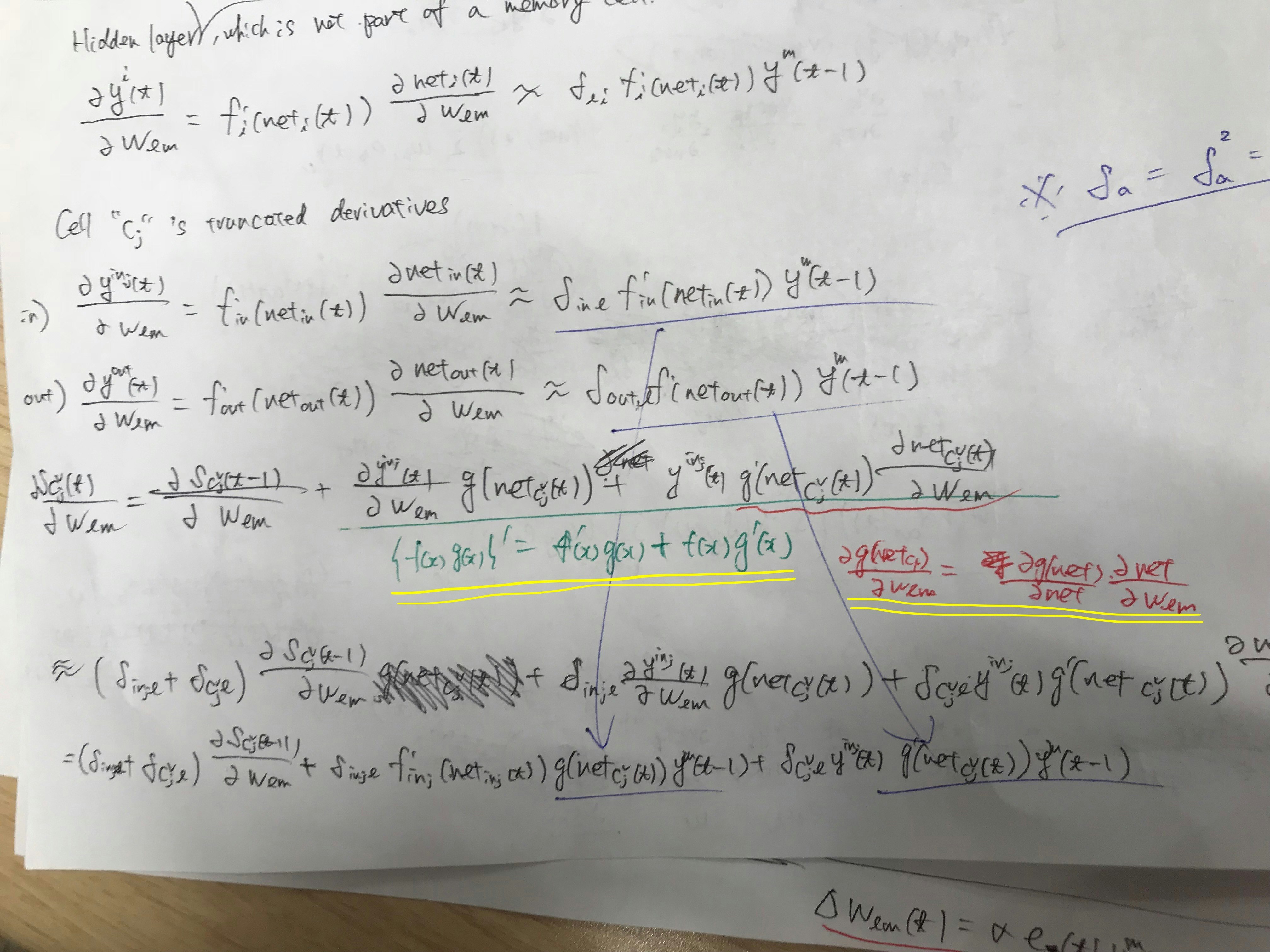
At first, the truncated derivatives of a hidden unit $i$ that is not a part of a memory cells are:

\frac{\partial y^i(t)}{\partial w_{lm}} = f'_i(net_i(t))\frac{\partial net^i(t)}{\partial w_{lm}} \approx_{tr} \delta_{li}f'_i(net_i(t))y^m(t-1)

Next, let's see inside the Cell block $c_j$ 's derivatives.

\begin{align}
\frac{\partial y^{in_j}(t)}{\partial w_{lm}} &= f'_{in_j}(net_{in_j}(t)) \frac{\partial net_{in_j}(t)}{\partial w_{lm}} \approx_{tr} \delta_{in_jl}f'_{in_j}(net_{in_j}(t))y^m(t-1)\\

\frac{\partial y^{out_j}(t)}{\partial w_{lm}} &= f'_{out_j}(net_{out_j}(t)) \frac{\partial net_{out_j}(t)}{\partial w_{lm}} \approx_{tr} \delta_{out_jl}f'_{out_j}(net_{out_j}(t))y^m(t-1)\\

\frac{\partial y^{c^v_j}(t)}{\partial w_{lm}} &= \frac{\partial y^{out_j}(t)}{\partial w_{lm}}h(s_{c^v_j}(t)) + h'(s_{c^v_j}(t))
 \frac{\partial s_{c^v_j}(t)}{\partial w_{lm}} y^{out_j}(t) \approx_{tr}
\delta_{out_jl} \frac{\partial y^{out_j}(t)}{\partial w_{lm}}h(s_{c^v_j}(t)) + \bigg(\delta_{in_j} + \delta_{c^v_j}\bigg) h'(s_{c^v_j}(t))
\frac{\partial s_{c^v_j}(t)}{\partial w_{lm}} y^{out_j}(t)\\

\frac{\partial s_{c^v_j}(t)}{\partial w_{lm}} &= \frac{\partial s_{c^v_j}(t-1)}{\partial w_{lm}} + \frac{\partial y^{in_j}(t)}{\partial w_{lm}}g \big (net_{c^v_j}(t) \big) + y^{in_j}(t) g' \big (net_{c^v_j}(t) \big)\frac{\partial net_{c^v_j}(t)}{\partial w_{lm}}\\
&\approx_{tr} \big( \delta_{in_jl} + \delta_{c^v_jl} \big) \frac{\partial s_{c^v_j}(t-1)}{\partial w_{lm}} + \delta_{in_jl} \frac{\partial y^{in_j}(t)}{\partial w_{lm}}g \big (net_{c^v_j}(t) \big) + \delta_{c^v_jl} y^{in_j}(t) g' \big (net_{c^v_j}(t) \big)\frac{\partial net_{c^v_j}(t)}{\partial w_{lm}}\\
&= \big( \delta_{in_jl} + \delta_{c^v_jl} \big) \frac{\partial s_{c^v_j}(t-1)}{\partial w_{lm}} + \delta_{in_jl} f'_{in_j}(net_{in_j}(t)) g \big (net_{c^v_j}(t) \big)y^m(t-1) + \delta_{c^v_jl} y^{in_j}(t) g' \big (net_{c^v_j}(t) \big)y^m(t-1)\\
\end{align}

Before jumping in, please remember that $E(t) = \sum_k (T^k(t) - y^k(t))^2$ where T means target, and y indicates output of LSTM.
Then we will define some unit l's error as below.

e_l(t) := -\frac{\partial E(t)}{\partial w_{lm}}

l = k (output) :

e_k(t) = -\frac{\partial E(t)}{\partial net_k(t)} = -\frac{\partial E}{\partial y}\frac{\partial y}{\partial net}\\
= f'_k(net_k(t))(T^k(t) - y^k(t))

l = i (hidden) :

e_i(t) = -\frac{\partial E(t)}{\partial net_i(t)} = -\frac{\partial E}{\partial y^k} \frac{\partial y^k}{\partial net_k} \frac{\partial net_k}{\partial y^i} \frac{\partial y^i}{\partial net_i}\\
= f'_i(net_i(t))\sum_{k: output unit}w_{ki}e_k(t)

l = $out_j$ (output gates)

e_{out_j}(t) = f'_{out_j}(net_{out_j}(t)) \bigg( \sum^{S_j}_{v=1}h(s_{c^v_j}(t)) 
\sum_{k: output unit}w_{kc^v_j}e_k(t) \bigg)

From now, let's dig into internal state $s_{c^v_j}$
l = $s_{c^v_j}$

e_{s_{c^v_j}} := -\frac{\partial E(t)}{\partial s_{c^v_j}} = -\frac{\partial E}{\partial y^k} \frac{\partial y^k}{\partial net_k} \frac{\partial net_k}{\partial y^{c^v_j}} \frac{\partial y^{c^v_j}}{\partial s_{c^v_j}}\\
= f_{out_j}(net_{out_j}(t))h'(s_{c^v_j}(t))\sum_{k:output unit}w_{kc^v_j}e_k(t)

4. SGD update for each weight matrix

SGD(Stochastic Gradient Descent) formulae

w_{t+1} ← w_t − η \frac{∂E(w_t)}{∂w_t}

Time t's contribution to $w_{lm}$'s gradient-based update with learning rate $\alpha$ is below.

\Delta w_{lm}(t) = - \alpha \frac{\partial E(t)}{\partial net_l(t)}\\
= \alpha \space e_l(t)y^m(t-1)

Let's see the details of updates
l = k (output) :

e_k(t) = f'_k(net_k(t))(T^k(t) - y^k(t))\\
\Delta  w_k = e_k(t)y^m(t-1)

l = i (hidden) :

e_i(t) = f'_i(net_i(t))\sum_{k: output unit}w_{ki}e_k(t)\\
\Delta  w_i = e_i(t)y^m(t-1)

l = $out_j$ (output gates)

e_{out_j}(t) = f'_{out_j}(net_{out_j}(t)) \bigg( \sum^{S_j}_{v=1}h(s_{c^v_j}(t)) 
\sum_{k: output unit}w_{kc^v_j}e_k(t) \bigg)\\
\Delta  w_{out_j} = e_{out_j}(t)y^m(t-1)

From now, let's dig into internal state $s_{c^v_j}$
l = $s_{c^v_j}$

e_{s_{c^v_j}} = f_{out_j}(net_{out_j}(t))h'(s_{c^v_j}(t))\sum_{k:output unit}w_{kc^v_j}e_k(t)\\
\Delta  w_{s_{c^v_j}} = e_{s_{c^v_j}}(t)y^m(t-1)

Then in order to obtain the gradient for input gate, we need to backpropagate more one!

-\frac{\partial E(t)}{\partial w_{lm}} = -\frac{\partial E(t)}{\partial s_{c^v_j}}\frac{\partial s_{c^v_j}}{\partial w_{lm}}\\
* -\frac{\partial E(t)}{\partial s_{c^v_j}} = -\frac{\partial E}{\partial y^k} \frac{\partial y^k}{\partial net_k} \frac{\partial net_k}{\partial y^{c^v_j}} \frac{\partial y^{c^v_j}}{\partial s_{c^v_j}} = e_{s_{c^v_j}}(t)\\
= \sum^{s_j}e_{s_{c^v_j}}(t) \frac{\partial s_{c^v_j}(t)}{\partial w_{lm}}\\
let \space l \space be \space in_j\\
* \frac{\partial s_{c^v_j}(t)}{\partial w_{in_jm}} = \frac{\partial s_{c^v_j}(t-1)}{\partial w_{in_jm}} + g(net_{c^v_j}(t))y^m(t-1);\\
* \Delta w_{in_jm}(t) = \alpha \sum^{s_j}e_{s_{c^v_j}}(t) \frac{\partial s_{c^v_j}(t)}{\partial w_{in_jm}}

Finally we have come back to the genuine input layer,

\frac{\partial s_{c^v_j}(t)}{\partial w_{c^v_jm}} = \frac{\partial s_{c^v_j}(t-1)}{\partial w_{c^v_jm}} + g'(net_{c^v_j}(t))f_{in_j}(net_{in_j}(t))y^m(t-1);\\
* \Delta w_{c^v_jm}(t) = \alpha e_{s_{c^v_j}}(t) \frac{\partial s_{c^v_j}(t)}{\partial w_{c^v_jm}}

素晴らしい記事

Additional Materials

Try implementation!
http://arunmallya.github.io/writeups/nn/lstm/index.html#/8
https://wiseodd.github.io/techblog/2016/08/12/lstm-backprop/