時系列解析手法のSARIMAモデルを試してみた #Python

製造業出身のデータサイエンティストがお送りする記事
今回は時系列解析手法のSARIMAモデルを試してみた

はじめに

過去に時系列解析に関しては何個か整理しておりますので、興味ある方は参照して頂けますと幸いです。

SARIMAモデルとは

SARIMAモデルを説明する前に、ARIMAモデルについて整理します。

ARIMAモデルとは、「autoregressive integrated moving average」の略で、自己回帰モデル(ARモデル)、移動平均モデル(MAモデル)、和分モデル(Iモデル)の3モデルを組み合わせたモデルです。

SARIMAモデルとは、「Seasonal AutoRegressive Integrated Moving Average」の略で、ARIMAモデルに「季節的な周期パターン」を加えたモデルです。
つまり、季節変動があるデータに対してARIMAモデルを拡張した手法が、SARIMAモデルです。具体的には、時系列方向にARIMAモデルを使い、かつ、周期方向にもARIMAモデルを使っているモデルです。

SARIMAモデル

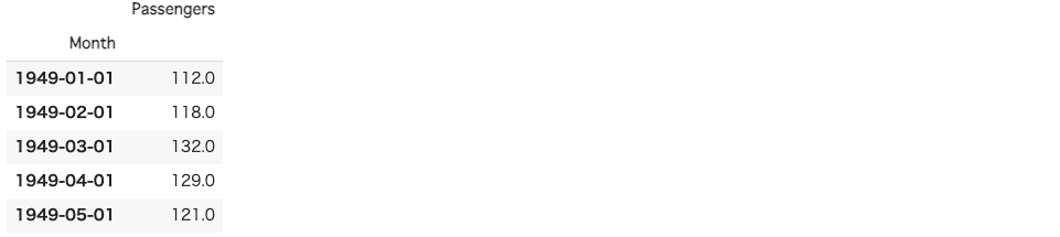
今回も使用したデータは、月ごとの飛行機の乗客数データです。

# ライブラリーのインポート
import warnings
warnings.filterwarnings('ignore')

import itertools

import matplotlib.pyplot as plt
import numpy as np
import pandas as pd
import statsmodels.api as sm
from plotly import tools
from plotly.graph_objs import Bar, Figure, Layout, Scatter
from plotly.offline import init_notebook_mode, iplot
from sklearn.metrics import mean_squared_error
from statsmodels.tsa.arima_model import ARIMA, ARMA
from statsmodels.tsa.statespace.sarimax import SARIMAX

import plotly
init_notebook_mode(connected=True)
save_image = None # 'png' if save image

# https://stat.ethz.ch/R-manual/R-devel/library/datasets/html/AirPassengers.html
df = pd.read_csv('../data/AirPassengers.csv')

# float型に変換
df['#Passengers'] = df['#Passengers'].astype('float64')
df = df.rename(columns={'#Passengers': 'Passengers'})

# datetime型にしてインデックスにする
df.Month = pd.to_datetime(df.Month)
df = df.set_index("Month")

# データの中身を確認
df.head()

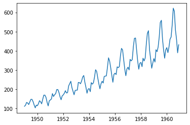
# データの可視化
plt.plot(df.Passengers)
plt.show()

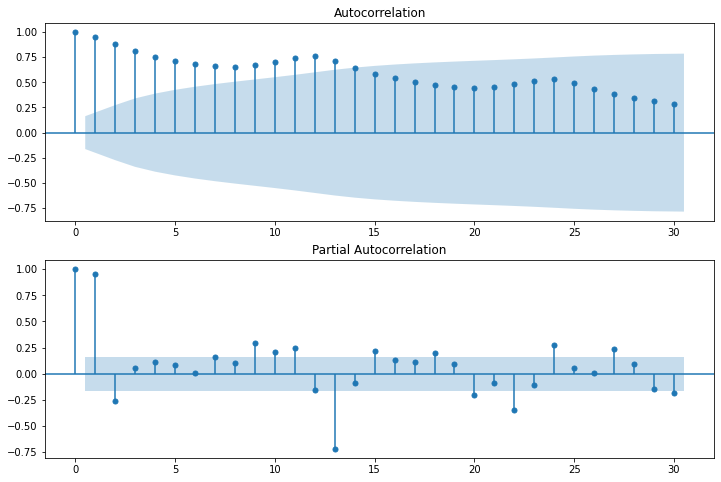
# コレログラム
fig = plt.figure(figsize=(12,8))
ax1 = fig.add_subplot(211)
fig = sm.graphics.tsa.plot_acf(df.Passengers, lags=30, ax=ax1)
ax2 = fig.add_subplot(212)
fig = sm.graphics.tsa.plot_pacf(df.Passengers, lags=30, ax=ax2)

次に定常性の確認を行います。
今回は、adfuller を用いて、Dickey-Fuller 検定を行いました。

res = sm.tsa.stattools.adfuller(df.Passengers)
print('p-value = {:.4}'.format(res[1]))
#p-value = 0.9919

Passengers: p-value > 0.1なので有意水準10%で帰無仮説（定常性を満たす）は棄却されず、定常ではない事が分かります。

次に、成分分解を行ってみます。

res = sm.tsa.seasonal_decompose(df["Passengers"])
fig = res.plot()

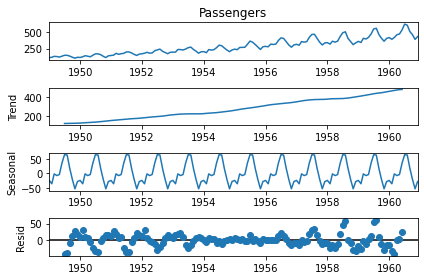
本当は差分系列や対数差分系列など、細かい確認が必要なのですが、今回はSARIMAモデルを試すことが重要なので進めます。
それでは、SARIMAモデルを構築します。

# 学習と評価データに分割
df_train = df[df.index < '1957-04-01']
df_test = df[df.index >= '1957-04-01']

ts = df.Passengers
ts_train = df_train.Passengers
ts_test = df_test.Passengers


def eval_model(ts_train, ts_test, result):
    train_pred = result.predict()
    test_pred = result.forecast(len(ts_test))
    test_pred_ci = result.get_forecast(len(ts_test)).conf_int()

    train_rmse = np.sqrt(mean_squared_error(ts_train, train_pred))
    test_rmse = np.sqrt(mean_squared_error(ts_test, test_pred))
    print('RMSE(train):\t{:.5}\nRMSE(test):\t{:.5}'.format(
        train_rmse, test_rmse))
    return train_pred, test_pred, test_pred_ci

order=(4,1,3)
seasonal_order=(1,1,1,12)
model = SARIMAX(
    ts_train,
    order=order,
    seasonal_order=seasonal_order,
    enforce_stationarity=False,
    enforce_invertibility=False)
result = model.fit()
train_pred, test_pred, test_pred_ci = eval_model(ts_train, ts_test, result)
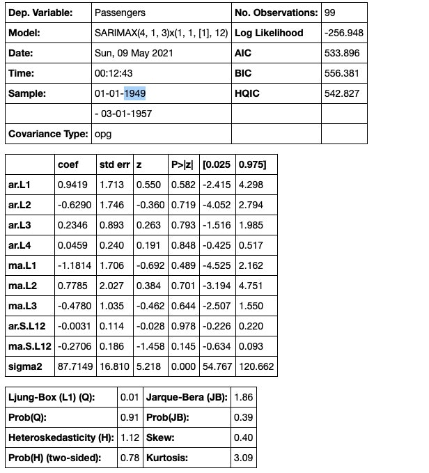
result.summary()

#RMSE(train):   17.811
#RMSE(test):    27.347

各パラメータは「arma_order_select_ic」などを用いて決めると良いと思います。

次は予測を行いたいと思います。

train_pred = result.predict()
test_pred = result.forecast(len(ts_test))
test_pred_ci = result.get_forecast(len(ts_test)).conf_int()

train_rmse = np.sqrt(mean_squared_error(df_train, train_pred))
test_rmse = np.sqrt(mean_squared_error(df_test, test_pred))
print('RMSE(train): {:.5}\nRMSE(test): {:.5}'.format(train_rmse, test_rmse))

#RMSE(train): 17.811
#RMSE(test): 27.347

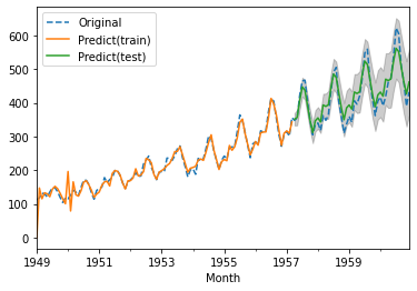
最後に可視化してみようと思います。

fig, ax = plt.subplots()
df.Passengers.plot(ax=ax, label='Original', linestyle="dashed")
train_pred.plot(ax=ax, label='Predict(train)')
test_pred.plot(ax=ax, label='Predict(test)')
ax.fill_between(
    test_pred_ci.index,
    test_pred_ci.iloc[:, 0],
    test_pred_ci.iloc[:, 1],
    color='k',
    alpha=.2)
ax.legend()

さいごに

最後まで読んで頂き、ありがとうございました。
時系列解析手法のSARIMAモデルを試してみた。

訂正要望がありましたら、ご連絡頂けますと幸いです。