概要

2014年6月18日、Colorado Rockies対Los Angeles Dodgersの試合でドジャースのClayton Kershaw投手は9回を投げ、15奪三振・ノーヒットノーランを達成しました。今回は対戦相手Rockiesの投手と比較し、なぜClayton Kershaw投手はノーヒットノーランを達成できたのか分析します。

環境

・Python 3.7.5
・windows10
・Jupyter Notebook(Anaconda3)

分析開始（プレイーボール）

まずはAnaconda PromptでJupyter Notebookを起動

$ jupyter notebook

続いて必要なライブラリをインポート

baseball_analysis.ipynb

%matplotlib inline  
import requests
import xml.etree.ElementTree as ET
import os
import pandas as pd

これから分析するためのデータフレームを作っていく

baseball_analysis.ipynb

# データフレーム作成
pitchDF = pd.DataFrame(columns = ['pitchIdx', 'inning', 'frame', 'ab', 'abIdx', 'batter', 'stand', 'speed', 
                                       'pitchtype', 'px', 'pz', 'szTop', 'szBottom', 'des'], dtype=object)

# 球種辞書作成
pitchDictionary = { "FA":"fastball", "FF":"4-seam fb", "FT": "2-seam fb", "FC": "fb-cutter", "":"unknown", None: "none",
                    "FS":"fb-splitter", "SL":"slider", "CH":"changeup","CU":"curveball","KC":"knuckle-curve",
                    "KN":"knuckleball","EP":"eephus", "UN":"unidentified", "PO":"pitchout", "SI":"sinker", "SF":"split-finger"
                    }

# top=表、bottom=裏
frames = ["top", "bottom"]

選手の情報の取得

baseball_analysis.ipynb

# MLB Advanced Mediaが配信しているプレイヤー情報を読み込み
url = 'https://gd2.mlb.com/components/game/mlb/year_2014/month_06/day_18/gid_2014_06_18_colmlb_lanmlb_1/players.xml'
resp = requests.get(url) 
xmlfile = "myplayers.xml"

with open(xmlfile, mode='wb') as f:
    f.write(resp.content)
statinfo = os.stat(xmlfile)

# xmlファイルを解析
tree = ET.parse(xmlfile)
game = tree.getroot()
teams = game.findall("./team")
playerDict = {}

for team in teams:
    players = team.findall("./player")
    for player in players:
        # プレイヤーIDと選手名を辞書に追加
        playerDict[ player.attrib.get("id") ] = player.attrib.get("first") + " " + player.attrib.get("last")

イニング毎のデータ取得

baseball_analysis.ipynb

# MLB Advanced Mediaが配信しているイニング毎のデータを読み込み
url = 'https://gd2.mlb.com/components/game/mlb/year_2014/month_06/day_18/gid_2014_06_18_colmlb_lanmlb_1/inning/inning_all.xml'
resp = requests.get(url) 
xmlfile = "mygame.xml"

with open(xmlfile, 'wb') as f: 
    f.write(resp.content)
statinfo = os.stat(xmlfile) 

# xmlファイルを解析
tree = ET.parse(xmlfile)
root = tree.getroot()
innings = root.findall("./inning")

totalPitchCount = 0
topPitchCount = 0
bottomPitchCount = 0

for inning in innings:
    for i in range(len(frames)):
        fr = inning.find(frames[i])
        if fr is not None:
            for ab in fr.iter('atbat'):
                battername = playerDict[ab.get('batter')]
                standside = ab.get('stand')
                abIdx = ab.get('num')
                abPitchCount = 0
                pitches = ab.findall("pitch")
                for pitch in pitches:
                    if pitch.attrib.get("start_speed") is None:
                        speed == 0
                    else:
                        speed = float(pitch.attrib.get("start_speed"))

                    pxFloat = 0.0 if pitch.attrib.get("px") == None else float('{0:.2f}'.format(float(pitch.attrib.get("px"))))
                    pzFloat = 0.0 if pitch.attrib.get("pz") == None else float('{0:.2f}'.format(float(pitch.attrib.get("pz"))))
                    szTop = 0.0 if pitch.attrib.get("sz_top") == None else float('{0:.2f}'.format(float(pitch.attrib.get("sz_top"))))
                    szBot = 0.0 if pitch.attrib.get("sz_bot") == None else float('{0:.2f}'.format(float(pitch.attrib.get("sz_bot"))))

                    abPitchCount = abPitchCount + 1
                    totalPitchCount = totalPitchCount + 1

                    if frames[i]=='top':
                        topPitchCount = topPitchCount + 1
                    else:
                        bottomPitchCount = bottomPitchCount + 1

                    inn = inning.attrib.get("num")

                    verbosePitch = pitchDictionary[pitch.get("pitch_type")]

                    desPitch = pitch.get("des")

                    # データフレームに追加
                    pitchDF.loc[totalPitchCount] = [float(totalPitchCount), inn, frames[i], abIdx, abPitchCount, battername, standside, speed,
                                               verbosePitch, pxFloat, pzFloat, szTop, szBot, desPitch]

データフレーム確認

baseball_analysis.ipynb

pitchDF

# pitchIdx=通し番号
# inning=イニング
# frame=裏表
# ab=打者ID
# abIdx=打席毎の球数
# batter=打者名
# stand=打席(R→右打ち、L→左打ち)
# speed=球速
# pitchtype=球種
# px=ホームベース通過位置(左右)(右→正、左→負)
# pz=ホームベース通過位置(高低)
# szTop=地面からバッターのストライクゾーンの最高値までの距離
# szBottom=地面からバッターのストライクゾーンの最低値までの距離
# des=結果

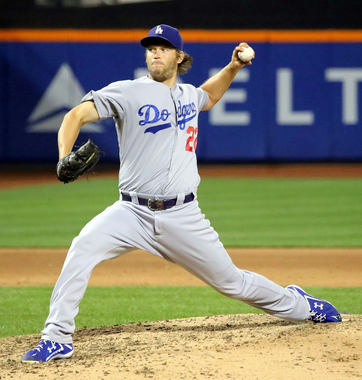
ストライクゾーン作成

baseball_analysis.ipynb

import matplotlib.pyplot as plt
import matplotlib.patches as patches

# 新規のウィンドウを描画
fig1 = plt.figure()
# subplotを追加
ax1 = fig1.add_subplot(111, aspect='equal')

# ストライクゾーン横幅は17インチ = 1.4フィート
# ストライクゾーン縦幅は1.5～3.5フィート
# 野球ボールのサイズは3インチ = 0.25フィート
# フィートの求め方 = インチ / 12

# ストライクゾーン作成
# 青のフレームはストライクゾーン
platewidthInFeet = 17 / 12
szHeightInFeet = 3.5 - 1.5

# ボール一個分外のストライクゾーン作成
# ライトブルーのフレームはボール一個分外のストライクゾーン
expandedPlateInFeet = 20 / 12
ballInFeet = 3 / 12
halfBallInFeet = ballInFeet / 2

ax1.add_patch(patches.Rectangle((expandedPlateInFeet/-2, 1.5 - halfBallInFeet), expandedPlateInFeet, szHeightInFeet + ballInFeet, color='lightblue'))
ax1.add_patch(patches.Rectangle((platewidthInFeet/-2, 1.5), platewidthInFeet, szHeightInFeet))

plt.ylim(0, 5)
plt.xlim(-2, 2)
plt.show()

データフレームにストライク・ボール判定を追加

baseball_analysis.ipynb

uniqDesList = pitchDF.des.unique()
ballColList = [] 
strikeColList = []
ballCount = 0
strikeCount = 0

for index, row in pitchDF.iterrows():
    des = row['des']
    if row['abIdx'] == 1:
        ballCount = 0
        strikeCount = 0

    ballColList.append(ballCount)
    strikeColList.append(strikeCount)

    if 'Ball' in des:
        ballCount = ballCount + 1
    elif 'Foul' in des:
        if strikeCount is not 2:
            strikeCount = strikeCount + 1
    elif 'Strike' in des:
        strikeCount = strikeCount + 1

# データフレームに追加
pitchDF['ballCount'] = ballColList
pitchDF['strikeCount'] = strikeColList

データフレーム確認

baseball_analysis.ipynb

pitchDF

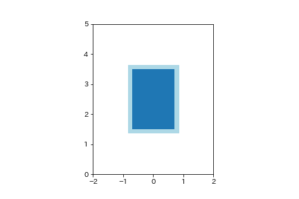
Clayton Kershaw(Dodgers)の投球傾向

baseball_analysis.ipynb

df= pitchDF.loc[pitchDF['frame']=='top']

ax1 = df.plot(kind='scatter', x='px', y='pz', marker='o', color='red', figsize=[8,8], ylim=[0,4], xlim=[-2,2])
ax1.set_xlabel('horizontal location')
ax1.set_ylabel('vertical location')
ax1.set_title('Clayton Kershawの投球傾向')
ax1.set_aspect(aspect=1)

platewidthInFeet = 17 / 12
expandedPlateInFeet = 20 / 12
szTop = df["szTop"].iloc[0]
szBottom = df["szBottom"].iloc[0]
szHeightInFeet = szTop - szBottom
ballInFeet = 3 / 12
halfBallInFeet = ballInFeet / 2

outrect = ax1.add_patch(patches.Rectangle((expandedPlateInFeet/-2, szBottom - halfBallInFeet), expandedPlateInFeet, szHeightInFeet + ballInFeet, color='lightblue'))
rect = ax1.add_patch(patches.Rectangle((platewidthInFeet/-2, szBottom), platewidthInFeet, szHeightInFeet))
outrect.zorder=-2 
rect.zorder=-1 

plt.ylim(0, 5)
plt.xlim(-2.5, 2.5)
plt.show()

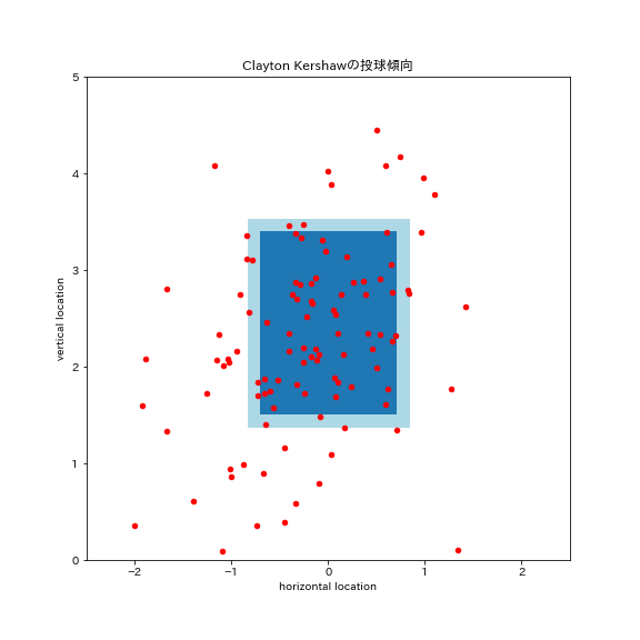
Rockiesの投球傾向

baseball_analysis.ipynb

df= pitchDF.loc[pitchDF['frame']=='bottom']

ax1 = df.plot(kind='scatter', x='px', y='pz', marker='o', color='red', figsize=[8,8], ylim=[0,4], xlim=[-2,2])
ax1.set_xlabel('horizontal location')
ax1.set_ylabel('vertical location')
ax1.set_title('Rockiesの投球傾向')
ax1.set_aspect(aspect=1)

platewidthInFeet = 17 / 12
expandedPlateInFeet = 20 / 12
szTop = df["szTop"].iloc[0]
szBottom = df["szBottom"].iloc[0]
szHeightInFeet = szTop - szBottom
ballInFeet = 3 / 12
halfBallInFeet = ballInFeet / 2

outrect = ax1.add_patch(patches.Rectangle((expandedPlateInFeet/-2, szBottom - halfBallInFeet), expandedPlateInFeet, szHeightInFeet + ballInFeet, color='lightblue'))
rect = ax1.add_patch(patches.Rectangle((platewidthInFeet/-2, szBottom), platewidthInFeet, szHeightInFeet))
outrect.zorder=-2 
rect.zorder=-1 

plt.ylim(0, 5)
plt.xlim(-2.5, 2.5)
plt.show()

両投手を比較してみると、
Claytonのストライク率: 65%
Rockiesのストライク率: 56%
だということが分かりました。
ClaytonはRockiesの投手と比べて、横への外れ球が少ない気がします。縦へのばらつきが多いのはスライダーの影響かorホップするストレート？

次は初球傾向を見てみます。

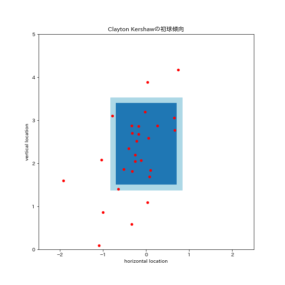
Clayton Kershaw(Dodgers)の初球傾向

baseball_analysis.ipynb

df= pitchDF.loc[pitchDF['frame']=='top'].loc[pitchDF['abIdx']==1]

ax1 = df.plot(kind='scatter', x='px', y='pz', marker='o', color='red', figsize=[8,8], ylim=[0,4], xlim=[-2,2])
ax1.set_xlabel('horizontal location')
ax1.set_ylabel('vertical location')
ax1.set_title('Clayton Kershawの初球傾向')
ax1.set_aspect(aspect=1)

platewidthInFeet = 17 / 12
expandedPlateInFeet = 20 / 12
szTop = df["szTop"].iloc[0]
szBottom = df["szBottom"].iloc[0]
szHeightInFeet = szTop - szBottom
ballInFeet = 3 / 12
halfBallInFeet = ballInFeet / 2

outrect = ax1.add_patch(patches.Rectangle((expandedPlateInFeet/-2, szBottom - halfBallInFeet), expandedPlateInFeet, szHeightInFeet + ballInFeet, color='lightblue'))
rect = ax1.add_patch(patches.Rectangle((platewidthInFeet/-2, szBottom), platewidthInFeet, szHeightInFeet))
outrect.zorder=-2 
rect.zorder=-1 

plt.ylim(0, 5)
plt.xlim(-2.5, 2.5)
plt.show()

Rockiesの初球傾向

baseball_analysis.ipynb

df= pitchDF.loc[pitchDF['frame']=='bottom'].loc[pitchDF['abIdx']==1]

ax1 = df.plot(kind='scatter', x='px', y='pz', marker='o', color='red', figsize=[8,8], ylim=[0,4], xlim=[-2,2])
ax1.set_xlabel('horizontal location')
ax1.set_ylabel('vertical location')
ax1.set_title('Rockiesの初球傾向')
ax1.set_aspect(aspect=1)

platewidthInFeet = 17 / 12
expandedPlateInFeet = 20 / 12
szTop = df["szTop"].iloc[0]
szBottom = df["szBottom"].iloc[0]
szHeightInFeet = szTop - szBottom
ballInFeet = 3 / 12
halfBallInFeet = ballInFeet / 2

outrect = ax1.add_patch(patches.Rectangle((expandedPlateInFeet/-2, szBottom - halfBallInFeet), expandedPlateInFeet, szHeightInFeet + ballInFeet, color='lightblue'))
rect = ax1.add_patch(patches.Rectangle((platewidthInFeet/-2, szBottom), platewidthInFeet, szHeightInFeet))
outrect.zorder=-2 
rect.zorder=-1 

plt.ylim(0, 5)
plt.xlim(-2.5, 2.5)
plt.show()

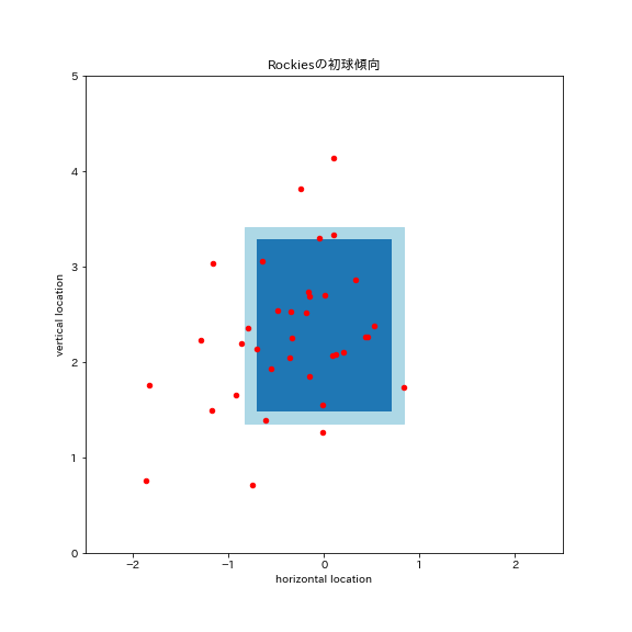
両投手を比較してみると、
Claytonの初球ストライク率: 71%
Rockiesの初球ストライク率: 64%
だということが分かりました。

Clayton投手は球数も少なくストライク先行してますね。

次は球速変化を見てみます。

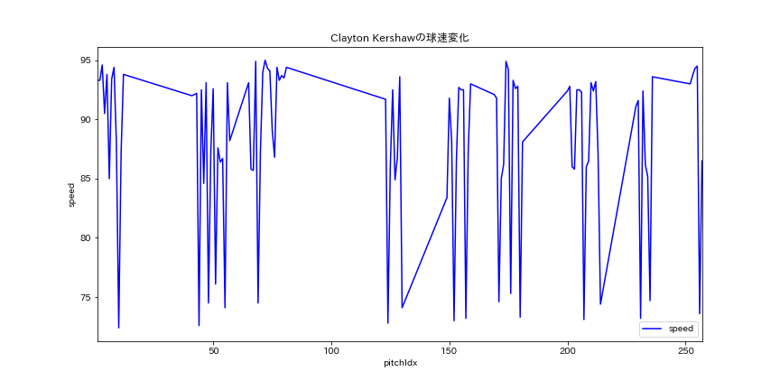
Clayton Kershaw(Dodgers)の球速変化

baseball_analysis.ipynb

df = pitchDF.loc[(pitchDF['frame']=='top')]

speed = df['speed']
print(sum(speed) / len(speed))
print(max(speed))
print(min(speed))
print(max(speed) - min(speed))

ax = df.plot(x='pitchIdx', y='speed', color='blue', figsize=[12,6])
ax.set_ylabel('speed')
ax.set_title('Rockiesの球速変化')
plt.savefig('pitch_rockies_speed.png')
plt.show()
>>>>>>>>>>>>>>>>>>>>>>>>>
# 平均球速: 87.88504672897201
# 最速: 95.0
# 最遅: 72.4
# 緩急差: 22.599999999999994

Rockiesの球速変化

baseball_analysis.ipynb

df = pitchDF.loc[(pitchDF['frame']=='bottom')]

speed = df['speed']
print(sum(speed) / len(speed))
print(max(speed))
print(min(speed))
print(max(speed) - min(speed))

ax = df.plot(x='pitchIdx', y='speed', color='blue', figsize=[12,6])
ax.set_ylabel('speed')
ax.set_title('Rockiesの球速変化')
plt.savefig('pitch_rockies_speed.png')
plt.show()
>>>>>>>>>>>>>>>>>>>>>>>>>
# 平均球速: 89.13599999999998
# 最速: 96.3
# 最遅: 71.8
# 緩急差: 24.5

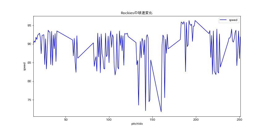
両投手を比較してみると、
Clayton
平均球速: 87マイル
最速: 95マイル
最遅: 72マイル
緩急差: 22マイル

Rockies
平均球速: 89マイル
最速: 96マイル
最遅: 71マイル
緩急差: 24マイル
だということが分かりました。

Rockiesは5人の投手を起用をしているので傾向に差がでるのは当たり前ですね。

次は球速変化を見てみます。

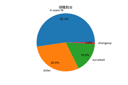
Clayton Kershaw(Dodgers)の球種割合

baseball_analysis.ipynb

df = pitchDF.loc[(pitchDF['frame']=='top')]

df.pitchtype.value_counts().plot(kind='pie', autopct="%.1f%%", pctdistance=0.8)
plt.axis('equal')
plt.axis('off')
plt.title('球種割合')
plt.show()

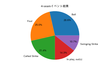
Clayton Kershaw(Dodgers)の4シームの結果

baseball_analysis.ipynb

df = pitchDF.loc[(pitchDF['pitchtype']=='4-seam fb') & (pitchDF['frame']=='top')]

df.des.value_counts().plot(kind='pie', autopct="%.1f%%", pctdistance=0.8)
plt.axis('equal')
plt.axis('off')
plt.title('4-seamイベント結果')
plt.show()

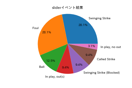
Clayton Kershaw(Dodgers)のスライダーの結果

baseball_analysis.ipynb

df = pitchDF.loc[(pitchDF['pitchtype']=='slider') & (pitchDF['frame']=='top')]

df.des.value_counts().plot(kind='pie', autopct="%.1f%%", pctdistance=0.8)
plt.axis('equal')
plt.axis('off')
plt.title('sliderイベント結果')
plt.show()

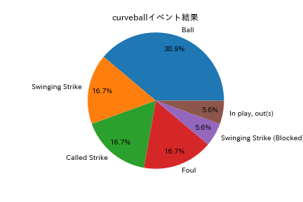
Clayton Kershaw(Dodgers)のカーブの結果

baseball_analysis.ipynb

df = pitchDF.loc[(pitchDF['pitchtype']=='curveball') & (pitchDF['frame']=='top')]

df.des.value_counts().plot(kind='pie', autopct="%.1f%%", pctdistance=0.8)
plt.axis('equal')
plt.axis('off')
plt.title('curveballイベント結果')
plt.show()

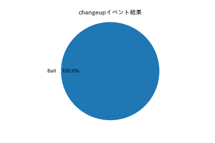
Clayton Kershaw(Dodgers)のチェンジアップの結果

baseball_analysis.ipynb

df = pitchDF.loc[(pitchDF['pitchtype']=='changeup') & (pitchDF['frame']=='top')]

df.des.value_counts().plot(kind='pie', autopct="%.1f%%", pctdistance=0.8)
plt.axis('equal')
plt.axis('off')
plt.title('changeupイベント結果')
plt.show()

球種毎のアウト率を比較してみると、
4シーム: 35.7%
スライダー: 18.8%
カーブ: 22.3%
チェンジアップ: 0%
だということが分かりました。

投球数の半分を占めるフォーシームでかなり打ち取ってますね。

次はカウント別配球を見てみます。

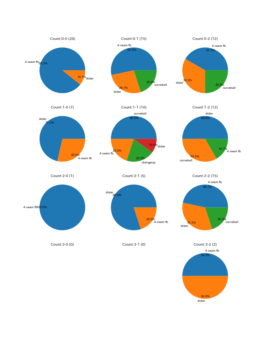
Clayton Kershaw(Dodgers)のカウント別配球

baseball_analysis.ipynb

titleList = []
dataList = []

fig, axes = plt.subplots(4, 3, figsize=(12,16))

# カウント作成
for b in range(4):
    for s in range(3):
        df = pitchDF.loc[(pitchDF['ballCount']==b) & (pitchDF['strikeCount']==s) & (pitchDF['frame']=='top')]
        title = "Count:" + str(b) + "-" + str(s) + " (" + str(len(df)) + ")"
        titleList.append(title)
        dataList.append(df)

for i, ax in enumerate(axes.flatten()):
    x = dataList[i].pitchtype.value_counts()
    l = dataList[i].pitchtype.unique()

    ax.pie(x, autopct="%.1f%%", pctdistance=0.9, labels=l)
    ax.set_title(titleList[i])

plt.show()

うーん、ほぼ4シーム。

次はカウント別結果を見てみます。

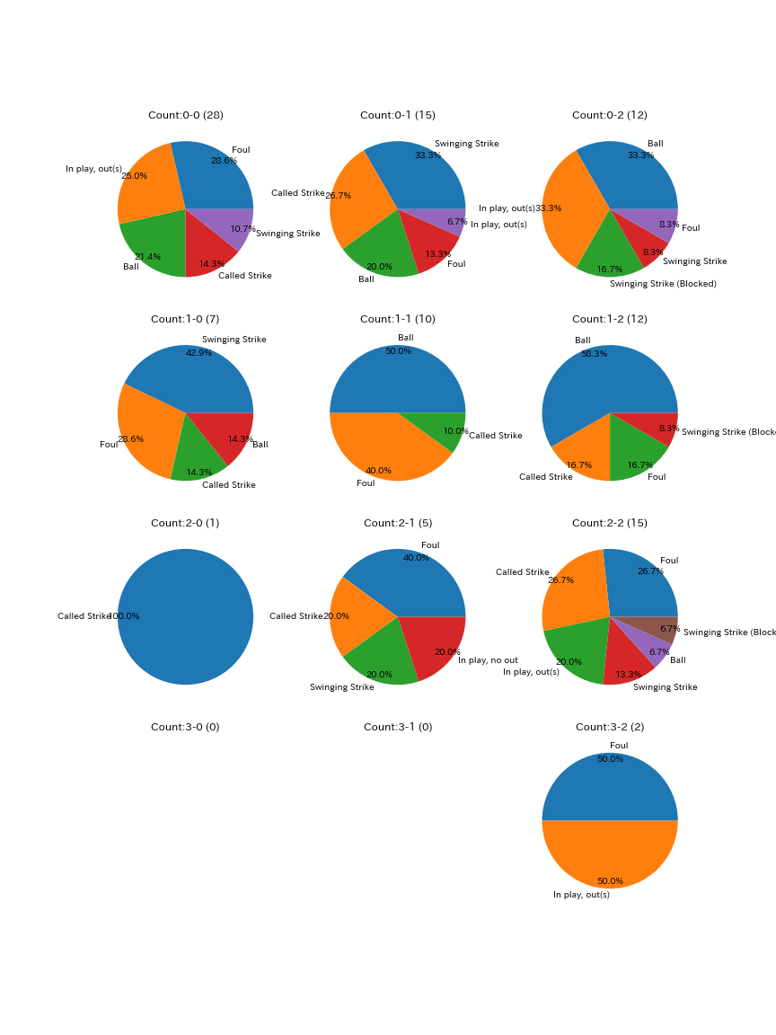
Clayton Kershaw(Dodgers)のカウント別結果

baseball_analysis.ipynb

titleList = []
dataList = []

fig, axes = plt.subplots(4, 3, figsize=(12,16))

for b in range(4):
    for s in range(3):
        df = pitchDF.loc[(pitchDF['ballCount']==b) & (pitchDF['strikeCount']==s) & pitchDF['des'] & (pitchDF['frame']=='top')]
        title = "Count:" + str(b) + "-" + str(s) + " (" + str(len(df)) + ")"
        titleList.append(title)
        dataList.append(df)

for i, ax in enumerate(axes.flatten()):
    x = dataList[i].des.value_counts()
    l = dataList[i].des.unique()

    ax.pie(x, autopct="%.1f%%", pctdistance=0.9, labels=l)
    ax.set_title(titleList[i])

plt.show()

どのカウントでもストライク判定、In play outs(フィールドにボールが飛んだ結果アウト)になる確率が高いのが分かりますね。

結論

初球ストライクが多く、有利なカウントを整えている（有利になる前に結構打ち取っている）
フォーシームの配球傾向が強い
不意にくるスライダーに注意（おそらく縦割れ系）

まとめ

Clayton投手の特徴はある程度熟知したが、なぜノーヒットノーランに至ったのかは他の試合と比較しないと明確な結果がわからなかった。また、対戦打者との過去対戦記録も必要になるだろう。Clayton投手はコントロールがよく、この試合の投球数はたった107球だった。MLBはNPBと比べて試合数が多く、中4日でシーズンを投げ通すため、仮にピッチャーが好投であっても投球制限で120球前後で降板させる傾向がある。そのため、メジャーでノーヒットノーランを達成にするにはコントロールの良さが最も重要な要因なのかもしれない。
長くなりましたが、ここまで読んでくださりありがとうございます。誤っている箇所がございましたら、コメントでご指摘頂けると大変嬉しいです。

【Python】ノーヒットノーランを成し遂げたピッチャーの分析をしてみた

概要

環境

分析開始（プレイーボール）

まずはAnaconda PromptでJupyter Notebookを起動

続いて必要なライブラリをインポート

これから分析するためのデータフレームを作っていく

選手の情報の取得

イニング毎のデータ取得

データフレーム確認

ストライクゾーン作成

データフレームにストライク・ボール判定を追加

データフレーム確認

Clayton Kershaw(Dodgers)の投球傾向

Rockiesの投球傾向

Clayton Kershaw(Dodgers)の初球傾向

Rockiesの初球傾向

Clayton Kershaw(Dodgers)の球速変化

Rockiesの球速変化

Clayton Kershaw(Dodgers)の球種割合

Clayton Kershaw(Dodgers)の4シームの結果

Clayton Kershaw(Dodgers)のスライダーの結果

Clayton Kershaw(Dodgers)のカーブの結果

Clayton Kershaw(Dodgers)のチェンジアップの結果

Clayton Kershaw(Dodgers)のカウント別配球

Clayton Kershaw(Dodgers)のカウント別結果

結論

まとめ