Kaggleコンペでトップ4%になった簡単ベイズ最適化

参加したコンペについて

参加したのはこちらのSwagコンペです。

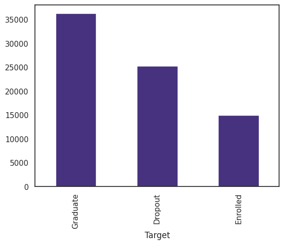
GDPや両親の学位など対象とする学生の周辺データからその学生の卒業、退学、その他の3つに分類するという課題です。

Swagは賞金がありませんが、Kaggleがホストするコンペで、この時は世界から2800人程度が参加しました。開催期間は1か月です。

私の順位は 107位 / 2684位 でした。
過学習を防ぐような工夫もしたので最後にグッと順位が上がりました。

SKF + LightGBM + BayesSearchCV

今回使ったモデルの構築方法はとてもコンパクトでお気に入りです。
コードは次の通りです。前処理が終わりモデルをつくる段階を想定してください。

from sklearn.model_selection import RepeatedStratifiedKFold
from sklearn.metrics import accuracy_score
from lightgbm import LGBMClassifier
from skopt import BayesSearchCV
from skopt.callbacks import DeadlineStopper, DeltaXStopper

params = {
    'num_leaves': Integer(32, 256, prior='uniform'),
    'learning_rate': Real(0.01, 0.1, prior='log-uniform'),
    'n_estimators': Integer(300, 2000, prior='uniform'),
    'subsample_for_bin': Integer(50000, 100000, prior='uniform'),
    'min_child_samples': Integer(50, 100, prior='uniform'),
    'reg_alpha': Real(1e-8, 1e-5, prior='log-uniform'),
    'reg_lambda': Real(1e-8, 1e-5, prior='log-uniform'),
    'colsample_bytree': Real(0.1, 0.9, prior='uniform'),
    'subsample': Real(0.5, 1.0, prior='uniform'),
    'max_depth': Integer(5, 8, prior='uniform')
}
skf = RepeatedStratifiedKFold(n_splits=10, n_repeats=3,random_state=42)

scoring = make_scorer(accuracy_score, greater_is_better=True, needs_proba=False)
opt = BayesSearchCV(
            LGBMClassifier(verbosity=-1,device='gpu'),
            params,
            scoring=scoring,
            cv=skf,
            n_iter=5000,
            n_jobs=1,  
            return_train_score=False,
            refit=True,
            optimizer_kwargs={'base_estimator': 'GP'},
            random_state=42
)

callbacks=[DeltaXStopper(0.001),DeadlineStopper(14400)]
opt.fit(X_train, y_train, callback=callbacks)
# best_score = opt.best_score_
# best_score_std = opt.cv_results_['std_test_score'][opt.best_index_]
# best_params = opt.best_params_
predicted = opt.predict(X_test)

1つずつ解説します。

BayesSearchCV

ハイパーパラメータの探索手法です。この手法とよく比較されるのはグリッドサーチです。
図のようなイメージです。
グリッドサーチは均等な間隔でパラメータを探索する手法ですが、探索回数が多く、時間がかかります。ベイズ最適化では局所解にスポットするのを防ぎつつ、それっぽいエリアを中心に探索します。

(この図だとベイズの方が点数は少ないですね...。)

理論はこちらの@meltyyyyyさんの記事がとても理解しやすく勉強になりました。

公式ドキュメントはこちらです。

RepeatedStratifiedKFold

StratifiedKFoldを指定した回数分行います。
StratifiedKFoldは通常のKFoldに比べてクラスラベルが均等に割り振られる手法です。

公式ドキュメントにわかりやすい図がありました。
赤い部分がテストデータで、StatifiedKFoldでは各クラスラベルから教師データとテストデータが分割されています。

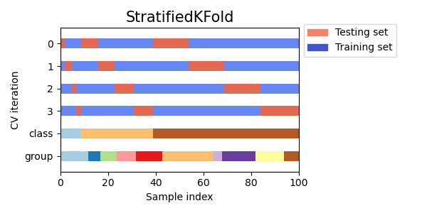
今回のデータでは、学生の中で卒業した人が最も多かったのでこのような手法を使いましたが、RepeatedKFoldを使っても良いと思います。

LightGBMと組み合わせる

LightGBMのインスタンスをBayesSearchCVの引数に渡し、LightGBMのパラメータ探索を行います。
パラメータには範囲を設定します。

params = {
   'n_estimators': Integer(300, 2000, prior='uniform'),
   'max_depth': Integer(5, 8, prior='uniform')
}

opt = BayesSearchCV(LGBMClassifier(), params)

続いて、BayesSearchCVの中にクロスバリデーションの戦略を定義します。こちらは任意のオプションです。

skf = RepeatedStratifiedKFold(n_splits=10, n_repeats=3,random_state=42)

params = {
   'n_estimators': Integer(300, 2000, prior='uniform'),
   'max_depth': Integer(5, 8, prior='uniform')
}

opt = BayesSearchCV(LGBMClassifier(), params, cv=skf)

fit()メソッドでモデルをつくり、そのまま推論モデルとして使えます。また、ベイズ最適化の結果として得られたパラメータも呼び出せます。

opt.fit(X_train, y_train)
best_params = opt.best_params_
predicted = opt.predict(X_test)

最終的なコードは記事の上部にあります！

コンペでの立ち回り

このコンペはSwagということもあり、あまり時間をかけずにスコアを上げることを期待しました。これだけシンプルでかなり安定したスコアが出るのは魅力的ですね。

おまけ

グリッドサーチとベイズ最適化の違いを示すコードはこちらです。

サンプル

import numpy as np
import matplotlib.pyplot as plt
from sklearn.model_selection import GridSearchCV
from skopt import BayesSearchCV
from skopt.space import Real
from sklearn.datasets import make_classification
from sklearn.svm import SVC

# サンプルデータセット
X, y = make_classification(n_samples=100, n_features=2, n_informative=2, n_redundant=0, random_state=42)

# サポートベクターマシンを対象のモデルにした
model = SVC()

# パラメータの範囲
param_grid = {'C': [0.1, 1, 10, 100], 'gamma': [1, 0.1, 0.01, 0.001]}
param_bayes = {'C': Real(0.1, 100, prior='log-uniform'), 'gamma': Real(0.001, 1, prior='log-uniform')}

# グリッドサーチ
grid_search = GridSearchCV(model, param_grid, cv=3)
grid_search.fit(X, y)

# グリッドサーチの探索点
grid_points = np.array([[params['C'], params['gamma']] for params in grid_search.cv_results_['params']])

# ベイズサーチ
bayes_search = BayesSearchCV(model, param_bayes, n_iter=30, cv=3, random_state=42)
bayes_search.fit(X, y)

# ベイズサーチの探索点
bayes_points = np.array([[result['C'], result['gamma']] for result in bayes_search.cv_results_['params']])

# 2次元プロット
fig, (ax1, ax2) = plt.subplots(1, 2, figsize=(14, 6))

# グリッドサーチのプロット
ax1.scatter(grid_points[:, 0], grid_points[:, 1], c='r', marker='o', label='Grid Search Points')
ax1.set_title('Grid Search')
ax1.set_xlabel('C')
ax1.set_ylabel('gamma')
ax1.set_xscale('log')
ax1.set_yscale('log')
ax1.legend()

# ベイズサーチのプロット
ax2.scatter(bayes_points[:, 0], bayes_points[:, 1], c='b', marker='o', label='Bayesian Search Points')
ax2.set_title('Bayesian Search')
ax2.set_xlabel('C')
ax2.set_ylabel('gamma')
ax2.set_xscale('log')
ax2.set_yscale('log')
ax2.legend()

plt.show()