0. はじめに

Kaggleなどで機械学習を用いて回帰・分類をする際のおおまかな流れは、
データの読み込み→欠損値処理→ラベルエンコーディング→
→EDA→ワンホットエンコーディング→
→ベースラインモデルの作成→複雑なモデルの構築→
→パラメーターチューニング
みたいな感じです。

その中でも、ベースラインモデルでの回帰・分類は割とパターンとして解けます。
さらに、そこにPipeline処理を用いることでより素早く解けます。
そこで、今回はベースラインモデルの構築、パイプライン処理についてまとめてみました。

1. 準備

今回用いたデータセットは、Kaggleに落ちているtitanicのデータセットです。

ワンホットエンコーディングまではこんな感じ。
ここまでの詳細は前回の記事にまとめています。

In[1]

%matplotlib inline
import matplotlib as plt
import pandas as pd
import numpy as np
import seaborn as sns
import collections

df = pd.read_csv('./train.csv')
df = df.set_index('PassengerId') #一意性がある列をindexに設定する
df = df.drop(['Name', 'Ticket'], axis=1) #分析に不要な列をdropする
df = df.drop(['Cabin'], axis=1) #分析には使いにくそうなので削除
df = df.dropna(subset = ['Embarked']) #Cabinは欠損が少ないのでdropnaで行を削除
df = df.fillna(method = 'ffill') #他の列は前のデータから補完

from sklearn.preprocessing import LabelEncoder
for column in ['Sex','Embarked']:
    le = LabelEncoder()
    le.fit(df[column])
    df[column] = le.transform(df[column])

df_continuous = df[['Age','SibSp','Parch','Fare']]

df = pd.get_dummies(df, columns = ['Pclass','Embarked'])
df.head()

次に、これをtrain_test_splitでtrainデータとtestデータに分割します。

In[2]

from sklearn.model_selection import train_test_split

X = df.drop(['Survived'], axis=1) 
y = df['Survived']

validation_size = 0.20
seed = 42 
X_train,X_test,y_train,y_test = train_test_split(X,y,test_size=validation_size,random_state=seed)

2. Baseline Modelの作成

Thanks: https://www.kaggle.com/mdiqbalbajmi/titanic-survival-prediction-beginner

必要なライブラリはこんな感じ。

In[3]

from sklearn.model_selection import KFold
from sklearn.model_selection import cross_val_score

from sklearn.neighbors import KNeighborsClassifier
from sklearn.discriminant_analysis import LinearDiscriminantAnalysis
from sklearn.naive_bayes import GaussianNB
from sklearn.svm import SVC
from sklearn.linear_model import LogisticRegression
from sklearn.tree import DecisionTreeClassifier

今回は、この6つのアルゴリズムをベースモデルとして用います。

Logistic回帰
線形判別
KNN(k近傍法)
CART(決定木)
ガウシアンナイーブベイズ
サポートベクターマシーン

また、KFoldによる交差検証を用いて、各モデルのスコアの分散も確認します。

In[4]


# Spot-check Algorithms
models = []

# In LogisticRegression set: solver='lbfgs',multi_class ='auto', max_iter=10000 to overcome warning
models.append(('LR',LogisticRegression(solver='lbfgs',multi_class='auto',max_iter=10000)))
models.append(('LDA',LinearDiscriminantAnalysis()))
models.append(('KNN',KNeighborsClassifier()))
models.append(('CART',DecisionTreeClassifier()))
models.append(('NB',GaussianNB()))
models.append(('SVM',SVC(gamma='scale')))

# evaluate each model in turn
results = []
names = []

for name, model in models:
    # initializing kfold by n_splits=10(no.of K)
    kfold = KFold(n_splits = 10, random_state=seed, shuffle=True) #crossvalidation

    # cross validation score of given model using cross-validation=kfold
    cv_results = cross_val_score(model,X_train,y_train,cv=kfold, scoring="accuracy")

    # appending cross validation result to results list
    results.append(cv_results)

    # appending name of algorithm to names list
    names.append(name)

    # printing cross_validation_result's mean and standard_deviation
    print(name, cv_results.mean()*100.0, "(",cv_results.std()*100.0,")")

出力はこんな感じ。

out[4]

LR 80.15845070422536 ( 5.042746503951439 )
LDA 79.31533646322379 ( 5.259067356458109 )
KNN 71.1658841940532 ( 3.9044128926316235 )
CART 76.50821596244131 ( 4.1506876372712815 )
NB 77.91471048513301 ( 4.426999157571688 )
SVM 66.9424882629108 ( 6.042153317290744 )

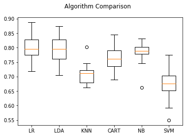
これを箱ひげ図で可視化します。

In[5]

figure = plt.figure()
figure.suptitle('Algorithm Comparison')
ax = figure.add_subplot(111)
plt.boxplot(results)
ax.set_xticklabels(names);

出力されたグラフがこちらです。

3. Pipeline処理

複数の処理がある時、それらの処理をパイプライン化しておくことでいくつか嬉しいことがあります。
コードが簡潔にできたり、GridSearchと組み合わせることでハイパーパラメーターの探索が簡単になったりなど。

Pipeline処理でできること

今回は、Standard Scaling(標準化)とモデルによる分類をパイプライン化してみます。

In[6]

# import pipeline to make machine learning pipeline to overcome data leakage problem
from sklearn.pipeline import Pipeline

# import StandardScaler to Column Standardize the data
# many algorithm assumes data to be Standardized
from sklearn.preprocessing import StandardScaler

# test options and evaluation matrix
num_folds=10
seed=42
scoring='accuracy'

# import warnings filter
from warnings import simplefilter
# ignore all future warnings
simplefilter(action='ignore', category=FutureWarning)

warningが出てくるので、そのまわりも対処しています。

ベースモデルごとにpipelineを構築し、それらをpipelinesに格納します。

In[7]

# source of code: machinelearningmastery.com
# Standardize the dataset
pipelines = []
pipelines.append(('ScaledLR', Pipeline([('Scaler', StandardScaler()),('LR',LogisticRegression(solver='lbfgs',multi_class='auto',max_iter=10000))])))
pipelines.append(('ScaledLDA', Pipeline([('Scaler', StandardScaler()),('LDA',LinearDiscriminantAnalysis())])))
pipelines.append(('ScaledKNN', Pipeline([('Scaler', StandardScaler()),('KNN',KNeighborsClassifier())])))
pipelines.append(('ScaledCART', Pipeline([('Scaler', StandardScaler()),('CART',DecisionTreeClassifier())])))
pipelines.append(('ScaledNB', Pipeline([('Scaler', StandardScaler()),('NB',GaussianNB())])))
pipelines.append(('ScaledSVM', Pipeline([('Scaler', StandardScaler()),('SVM', SVC(gamma='scale'))])))
results = []
names = []
for name, model in pipelines:
    kfold = KFold(n_splits=num_folds, random_state=seed)
    cv_results = cross_val_score(model, X_train, y_train, cv=kfold, scoring=scoring)
    results.append(cv_results)
    names.append(name)
    msg = "%s: %f (%f)" % (name, cv_results.mean()*100, cv_results.std())
    print(msg)

出力がこちらです。

out[7]

ScaledLR: 79.743740 (0.029184)
ScaledLDA: 79.045383 (0.042826)
ScaledKNN: 82.838419 (0.031490)
ScaledCART: 78.761737 (0.028512)
ScaledNB: 77.779734 (0.037019)
ScaledSVM: 82.703443 (0.029366)

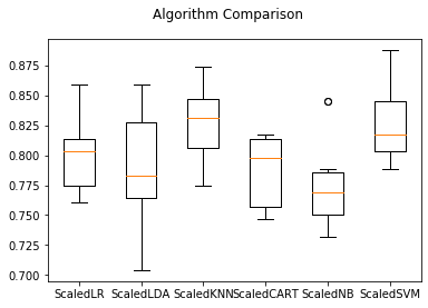
これを箱ひげ図にプロットします。

In[8]

# Compare Algorithms
fig = plt.figure()
fig.suptitle('Algorithm Comparison')
ax = fig.add_subplot(111)
plt.boxplot(results)
ax.set_xticklabels(names)
plt.show()

出力されたグラフはこの通り。

4. まとめ

ベースラインモデルの構築、パイプライン処理についてまとめてみました。
パイプライン処理は中々奥が深そうですね。

記事ネタ、コメントなど随時募集中です。

【Kaggle】Baseline modelの構築、Pipeline処理

0. はじめに

1. 準備

2. Baseline Modelの作成

3. Pipeline処理

4. まとめ