分析に使いづらい Excel を pandas で読む

Posted at 2026-04-30

Excel を pandas で読もうとして、こんな経験はないでしょうか。

import pandas as pd
df = pd.read_excel('fies_t1.xlsx')
df.head()

   Unnamed: 0  Unnamed: 1  Unnamed: 2  ...  Unnamed: 36
0         NaN         NaN         NaN  ...          NaN
1         NaN         NaN  月\nmonth   ...          NaN
2         NaN         NaN         NaN  ...          NaN
3         NaN         NaN         NaN  ...          NaN
4         NaN         NaN         NaN  ...          NaN

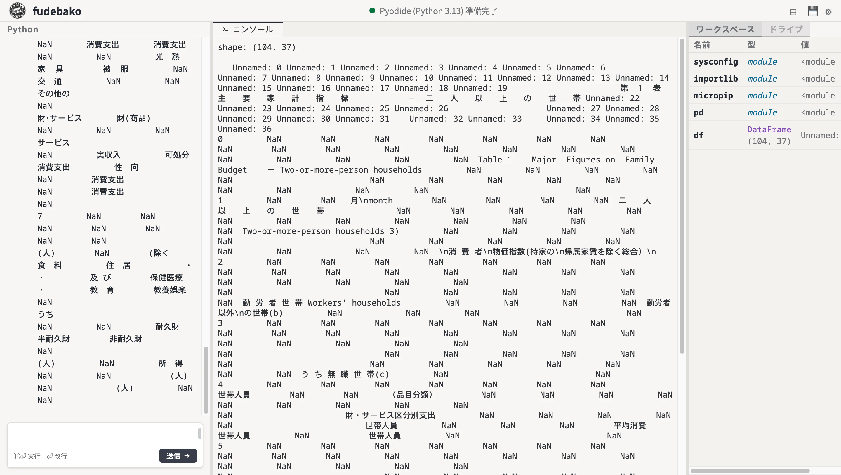
Unnamed: 0 が並び、上から 14 行ぐらい NaN だらけ。ヘッダーらしきものはセルをまたいで配置されています。header= を 1 や 2 に変えても、結局どこかで崩れる。よくある光景です。

これ、人間には読みやすいんですが、プログラムから見るとただの罠です。原因は merged cell（セル結合）と複数段ヘッダー。pd.read_excel が想定している「1 行目がカラム名、2 行目からデータ」という構造に真っ向から反しています。とはいえ、CSV が用意されていないデータも多く、Excel をそのまま整形するしか道がないこともあります。

この記事では、家計調査と消費者物価指数（CPI）の Excel を題材に、openpyxl で 1 セルずつ覗き込みながら DataFrame に変換する手順をメモしておきます。実行環境はブラウザだけで動く Python REPL の fudebako を使います。会社の PC に Python が入っていなくても、ブラウザのタブさえあれば完結します。

なお、私は fudebako の開発に関わっています。

この記事で扱うこと

pd.read_excel 一発では読めない Excel の構造を知る
openpyxl で生のセルを覗き、構造を物理的に把握する
merged cell の残骸（ffill）、複数段ヘッダー、年月混在カラムの整形
家計調査と CPI を結合して「実質消費支出」を可視化する

最後に可視化もしていますが、主役は Excel を REPL で少しずつ読み解いていくプロセスです。

準備：fudebako に Excel を読み込ませる

fudebako を開きます。HTML 1 枚で動く Pyodide ベースの Python REPL で、インストール不要、ファイルもブラウザ内（IndexedDB）で完結します。

統計局の家計調査月次データ fies_t1.xlsx を家計調査月次からダウンロードしておきます。

fudebako の Drive タブ から「+ インポート」、もしくはファイルを Drag & Drop で投入します。これで /drive/fies_t1.xlsx として Python から読めるようになります。

pandas / openpyxl / matplotlib は最初から入っているので、追加インストールは不要です。

もし同梱されていない wheel が必要な場合は、セルに %pip install パッケージ名 と書けばインストールできます（例：%pip install pypdf）。

§1. まず `pd.read_excel` で読んでみる（読めない）

とりあえず、普通に読んでみます。まあ、ダメなんですけど。

import pandas as pd
df = pd.read_excel('/drive/fies_t1.xlsx')
print(df.shape)
df.head(8)

(104, 37)

行数 104、列数 37。一見データはあるように見えますが、中身は冒頭で見た通り Unnamed の列が並び、最初の 8 行ぐらいは NaN だらけです。

header=1 や header=[0, 1, 2] も試せますが、merged cell のせいでヘッダーの位置がズレており、どれもうまくいきません。

ここで方針を切り替えます。ヘッダーを推測させるのを諦めて、header=None で生の値だけ読み込み、必要な行と列を自分で指定する。その前に、Excel の物理的な構造を目で確認します。

§2. openpyxl で生のセルを覗く

こういう時は openpyxl の出番です。pandas より低いレイヤーで、merged cell の情報もそのまま持っています。

import openpyxl
wb = openpyxl.load_workbook('/drive/fies_t1.xlsx', data_only=True)
print(wb.sheetnames)

['表１']

シートは「表１」だけ。これを開きます。

ws = wb['表１']
print(f'max_row={ws.max_row}, max_column={ws.max_column}')

max_row=106, max_column=38

106 行 × 38 列。さっき pandas で見た (104, 37) とほぼ同じですが、openpyxl の方は 1 行/列ぶん大きく出ています。pandas が空行を詰めて読むためです。

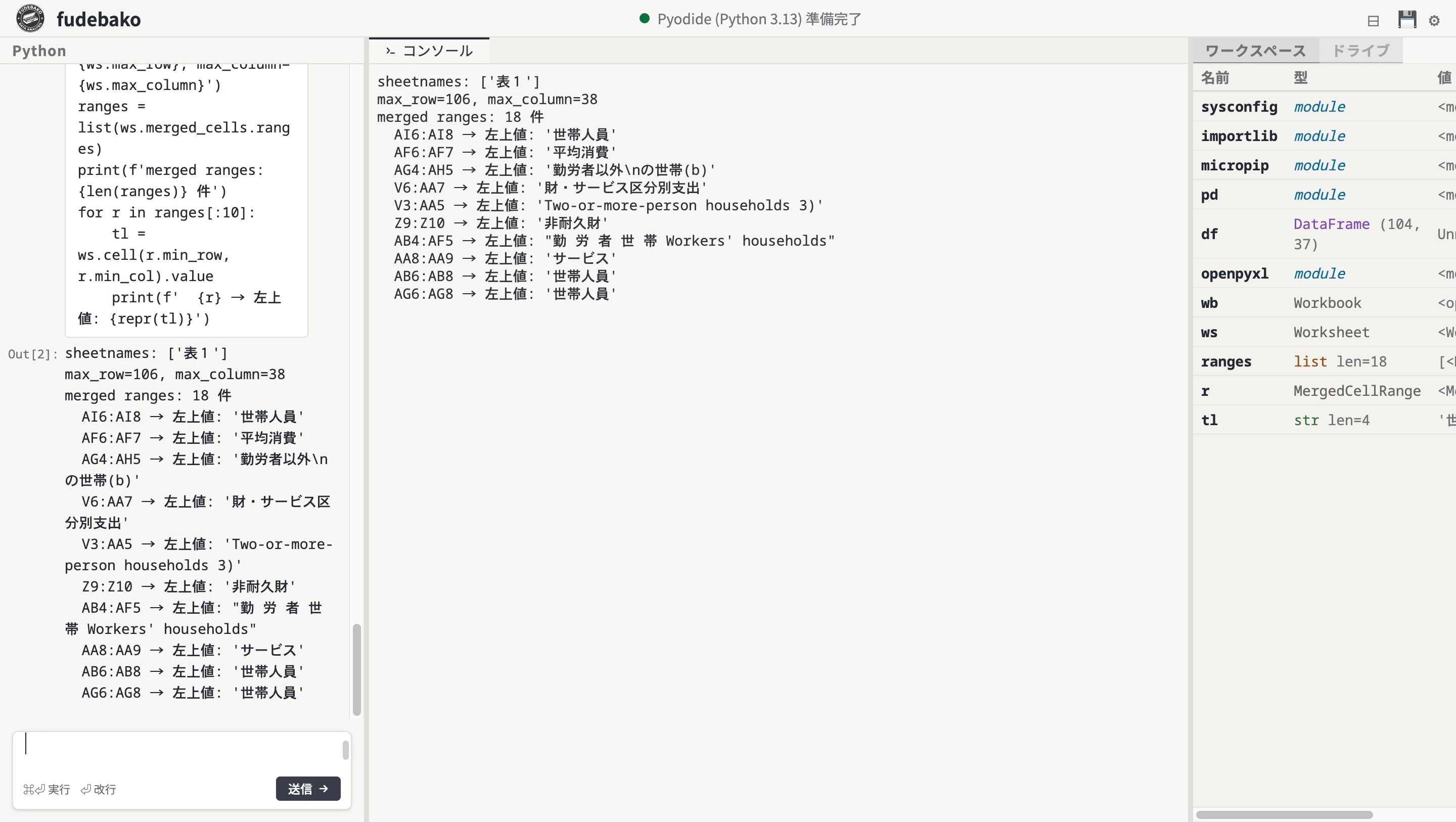
次に merged cell（セル結合）の場所を列挙してみます。

ranges = list(ws.merged_cells.ranges)
print(f'合計 {len(ranges)} 件')
for r in ranges[:10]:
    tl = ws.cell(r.min_row, r.min_col).value
    print(f'  {r} → 左上値: {repr(tl)}')

合計 18 件
  AF6:AF7 → 左上値: '平均消費'
  AB4:AF5 → 左上値: "勤 労 者 世 帯 Workers' households"
  AG4:AH5 → 左上値: '勤労者以外\nの世帯(b)'
  AB6:AB8 → 左上値: '世帯人員'
  V3:AA5 → 左上値: 'Two-or-more-person households 3)'
  AI6:AI8 → 左上値: '世帯人員'
  Y9:Y10 → 左上値: '半耐久財'
  Z9:Z10 → 左上値: '非耐久財'
  V6:AA7 → 左上値: '財・サービス区分別支出'
  AA8:AA9 → 左上値: 'サービス'

18 個の merged ranges。ヘッダーが複数列・複数行にまたがって 1 つのセルとして扱われています。これを pd.read_excel に正しく解釈しろ、というのは酷な話です。

§3. データの開始位置を見つける

ヘッダー領域をパースするのは早々に諦めて、データだけ抜き出す作戦にいきます。

どこから実データが始まっているのか、12 〜 18 行目あたりを 1 行ずつ覗いてみます（openpyxl は 1-indexed です）。

for r in range(12, 19):
    cells = [ws.cell(r, c).value for c in range(1, 11)]
    print(f'r{r:>3}: {cells}')

r 12: [None, None, None, None, None, None, None, 'household', 'Consumption', '(a)']
r 13: [None, None, None, None, None, None, None, '(persons)', 'expenditures', None]
r 14: [None, None, None, None, None, None, None, '　　...実　数（円）...', None, None]
r 15: [None, None, None, '2024年', '２', '月', '2024 Feb.', 2.89, 279868, 246720]
r 16: [None, None, None, '', '３', '', '     Mar.', 2.89, 318713, 273842]
r 17: [None, None, None, '', '４', '', '     Apr.', 2.88, 313300, 273702]
r 18: [None, None, None, '', '５', '', '     May', 2.88, 290328, 255295]

row 15 から実データが始まることがわかりました。列の意味も見えてきます。

col 4 = 年（「2024年」、それ以降は空文字 ''）
col 5 = 月（全角の「２」「３」「４」）
col 9 = 消費支出の円ベース値（279868 とか）

今回欲しいのは月次の消費支出なので、col 4 / 5 / 9 だけあれば十分です。

メモ: row 15 col 4 は '2024年' ですが、row 16 以降は '' です。これは Excel 上で merged cell になっているから。見た目は「2024年」が縦に伸びていますが、実体は左上のセルにしか値がありません。これが後で ffill が必要になる理由です。

§4. 必要な行と列を抜き出して整形する

ここからは pandas に戻ります。header=None で読み直して、iloc で row 15 以降（0-indexed なので iloc[14:]）を抜き出します。

df = pd.read_excel('/drive/fies_t1.xlsx', sheet_name='表１', header=None)
data = df.iloc[14:, [3, 4, 8]].copy()
data.columns = ['year', 'month', 'expenditure']
data.head()

     year month expenditure
14  2024年    ２      279868
15    NaN    ３      318713
16    NaN    ４      313300
17    NaN    ５      290328
18    NaN    ６      280888

ようやくそれっぽくなってきました。あとは細かいところを詰めます。

1. 年の merged 残骸を埋める
merged の名残で NaN が並んでいるので、ffill で前の値（'2024年'）を埋めます。

data['year'] = data['year'].ffill()

2. 「年」「月」を取り除いて数値化
全角の「２」も int() で 2 になるので、単純に astype(int) でいけます。

data['year'] = data['year'].astype(str).str.replace('年', '').astype(int)
data['month'] = data['month'].astype(str).str.replace('月', '').astype(int)

3. 金額データだけ残す
消費支出列には％基準の表なども混ざっているので、明らかに金額っぽい値（1000 以上）だけ残して掃除します。

data['expenditure'] = pd.to_numeric(data['expenditure'], errors='coerce')
data = data[data['expenditure'] > 1000].dropna()

4. datetime インデックスの作成

data['ym'] = pd.to_datetime(dict(year=data['year'], month=data['month'], day=1))
kakei = data[['ym', 'expenditure']].sort_values('ym').reset_index(drop=True)
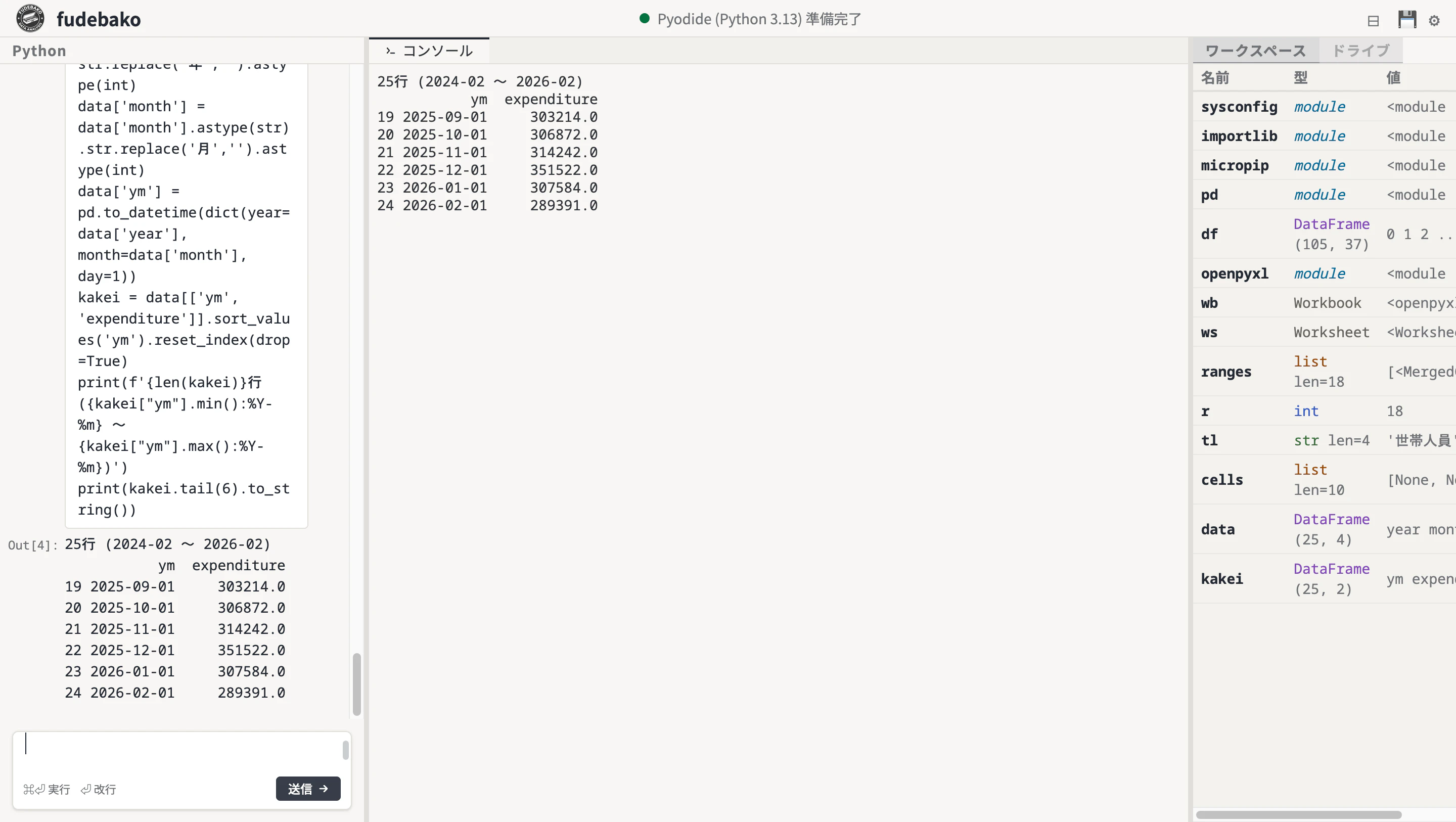
print(f'{len(kakei)}行 ({kakei["ym"].min():%Y-%m} 〜 {kakei["ym"].max():%Y-%m})')
kakei.tail(6)

25行 (2024-02 〜 2026-02)
          ym  expenditure
19 2025-09-01     303214.0
20 2025-10-01     306872.0
21 2025-11-01     314242.0
22 2025-12-01     351522.0
23 2026-01-01     307584.0
24 2026-02-01     289391.0

月次の消費支出が pandas DataFrame になりました。直近 2 年で月平均 30 万円前後。
Excel 整形の基本パターンは見えたので、次は CPI の Excel にも同じ手順を当ててみます。

§5. 同じ手順で CPI（列数 91 の大物 Excel）

消費者物価指数（CPI）の中分類指数を e-Stat から落とします。ファイル名は am01-1.xlsx。これも fudebako の Drive に放り込みます。

まずは openpyxl で構造をチェック。

wb2 = openpyxl.load_workbook('/drive/am01-1.xlsx', data_only=True)
ws2 = wb2['am01-1']
print(f'max_row={ws2.max_row}, max_column={ws2.max_column}')
print(f'merged: {len(list(ws2.merged_cells.ranges))} 件')

max_row=699, max_column=92
merged: 62 件

699 行 × 92 列、merged 62 件。なかなかの大物です。1970 年からの月次データに中分類 91 種類。

データ開始位置を確認。

for r in range(12, 21):
    cells = [ws2.cell(r, c).value for c in range(7, 12)]
    print(f'r{r:>3}: {cells}')

r 12: [None, None, 'All items', 'All items, less fresh food', 'All items, less imputed rent']
r 13: [None, 'ウエイト\n(2020年指数以降)', 10000, 9604, 8420]
r 14: [None, '品目数\n(2020年指数以降)', 582, 522, 581]
r 15: [None, '1970年 1月', 30.3, 30.5, 30.5]
r 16: [None, '2  ', 30.3, 30.6, 30.7]
r 17: [None, '3  ', 30.6, 30.6, 30.9]
r 18: [None, '4  ', 30.9, 30.9, 31.2]

row 15 からデータ開始なのは同じ。年月列は col 8（H 列）ですが、書き方が独特です。

1 月だけ '1970年 1月' と年が入っている
2 月以降は '2 ' のように月だけ（末尾に空白付き）
年は merged で先頭にしか書かれていない

「年だけ ffill して、月はそのまま使う」処理を組む必要があります。

中分類列の対応表を作って抜き出します（col 9 が総合、以降は食料、住居など）。

import re
df2 = pd.read_excel('/drive/am01-1.xlsx', sheet_name='am01-1', header=None)
col_map = {8: '総合', 14: '食料', 32: '住居', 39: '光熱・水道'}
md = df2.iloc[14:, [7] + list(col_map.keys())].copy()
md.columns = ['ym_str'] + list(col_map.values())
md.head()

      ym_str    総合    食料    住居  光熱・水道
14  1970年 1月  30.3  28.2  25.4   30.2
15        2   30.3  28.4  25.5   30.2
16        3   30.6  28.8  25.7   30.3
17        4   30.9  29.0  26.0   30.4
18        5   30.8  28.5  26.2   30.3

この ym_str をパースします。

def parse_ym(s):
    s = str(s).strip()
    m = re.match(r'(\d{4})年\s*(\d+)?月?', s)
    if m and m.group(2): return int(m.group(1)), int(m.group(2))
    if m: return int(m.group(1)), None     # 「1970年」だけ（年平均行）
    if s.isdigit() and 1 <= int(s) <= 12: return None, int(s)  # 月のみ
    return None, None

parsed = md['ym_str'].apply(parse_ym)
md['year'] = [p[0] for p in parsed]
md['month'] = [p[1] for p in parsed]
md['year'] = md['year'].ffill()           # 年を ffill で埋める
md = md[md['month'].notna()].copy()       # 年平均行（月が None）を除外
md['year'] = md['year'].astype(int)
md['month'] = md['month'].astype(int)
md['ym'] = pd.to_datetime(dict(year=md['year'], month=md['month'], day=1))
for c in col_map.values():
    md[c] = pd.to_numeric(md[c], errors='coerce')
cpi = md[['ym'] + list(col_map.values())].dropna().sort_values('ym').reset_index(drop=True)
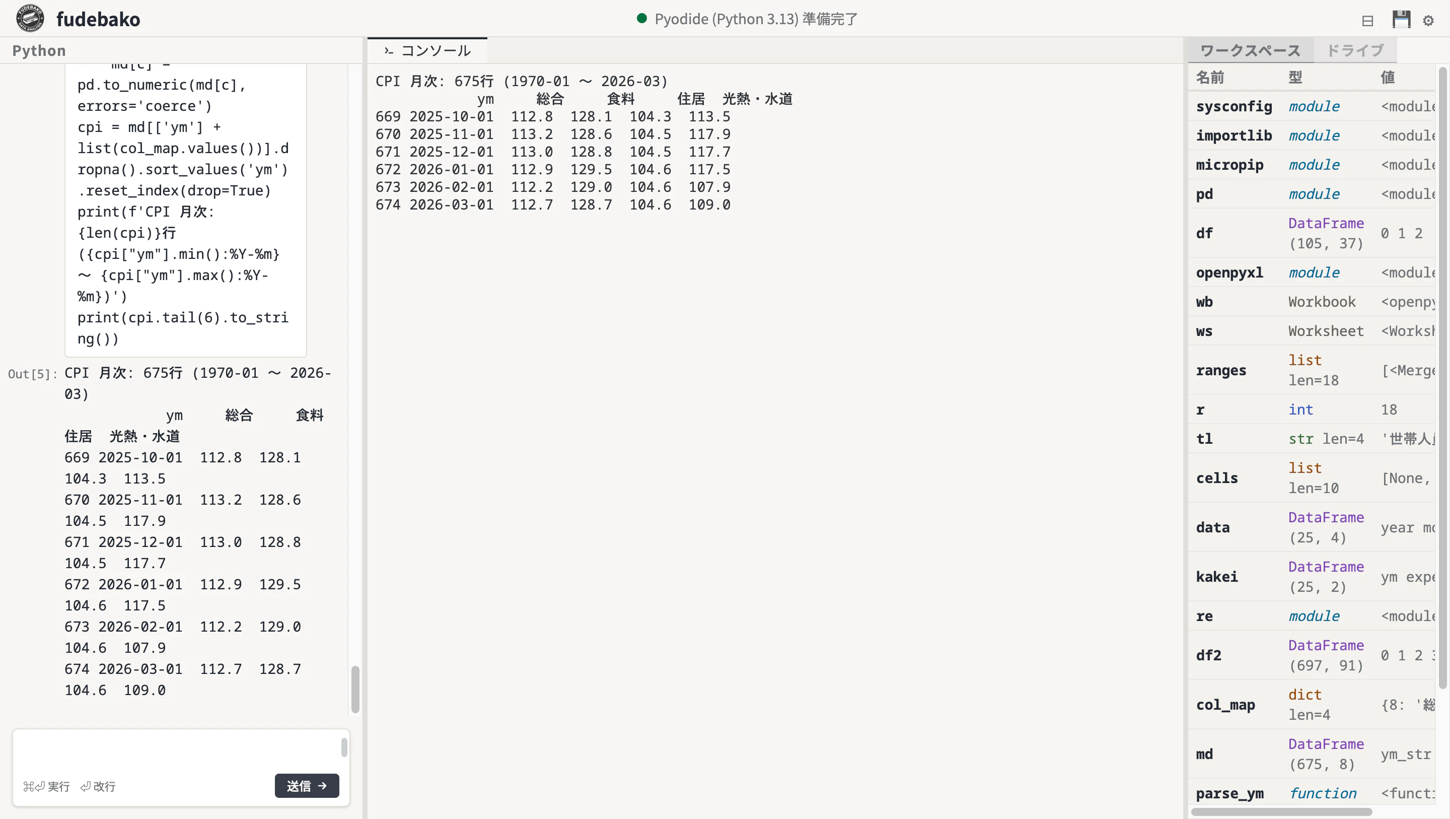
print(f'CPI 月次: {len(cpi)}行 ({cpi["ym"].min():%Y-%m} 〜 {cpi["ym"].max():%Y-%m})')
cpi.tail(6)

CPI 月次: 675行 (1970-01 〜 2026-03)
            ym     総合     食料     住居  光熱・水道
669 2025-10-01  112.8  128.1  104.3   113.5
670 2025-11-01  113.2  128.6  104.5   117.9
671 2025-12-01  113.0  128.8  104.5   117.7
672 2026-01-01  112.9  129.5  104.6   117.5
673 2026-02-01  112.2  129.0  104.6   107.9
674 2026-03-01  112.7  128.7  104.6   109.0

1970 年から 2026 年まで、675 行。長期データが取れました。

§6. 結合してプロット：物価で割って実質を出す

ようやく本題。家計調査と CPI を結合します。共通期間は 25 ヶ月分。

df = kakei.merge(cpi[['ym', '総合']], on='ym', how='inner')
df['real'] = df['expenditure'] / df['総合'] * 100  # 実質消費 = 名目 / CPI * 100
df['nominal_idx'] = df['expenditure'] / df['expenditure'].iloc[0] * 100
df['real_idx'] = df['real'] / df['real'].iloc[0] * 100
df.tail(6)[['ym', 'expenditure', '総合', 'real', 'nominal_idx', 'real_idx']]

            ym  expenditure     総合       real  nominal_idx  real_idx
19  2025-09-01       303214  112.0  270726.79       108.34    103.41
20  2025-10-01       306872  112.8  272049.65       109.65    103.91
21  2025-11-01       314242  113.2  277598.94       112.28    106.03
22  2025-12-01       351522  113.0  311081.42       125.60    118.82
23  2026-01-01       307584  112.9  272439.33       109.90    104.06
24  2026-02-01       289391  112.2  257924.24       103.40     98.52

2026 年 2 月の値を見ると、名目では +3.4% 増えていますが、CPI が +5.0% 上がっているせいで、実質では -1.5%。物価上昇に追いつかず、「使えるお金」は 2 年前を下回っています。

可視化します。fudebako のプロットタブはブラウザのフォントを使うので、日本語ラベルがそのまま表示されます（japanize-matplotlib は不要）。画像で保存したい場合は、プロットタブの ↓ ボタンからダウンロードしてください。

import matplotlib.pyplot as plt

fig, ax = plt.subplots(figsize=(10, 5))
ax.plot(df['ym'], df['nominal_idx'], label='名目（円ベース）',
        color='#d62728', marker='o', linewidth=2)
ax.plot(df['ym'], df['real_idx'], label='実質（CPI で割り戻し）',
        color='#1f77b4', marker='s', linewidth=2, linestyle='--')
ax.axhline(100, color='black', linewidth=0.6, linestyle=':')
ax.set_ylabel('インデックス（2024-02 = 100）')
ax.set_title('物価上昇下の家計支出：名目 vs 実質', fontsize=13)
ax.legend()
ax.grid(alpha=0.3)
plt.tight_layout()
plt.show()

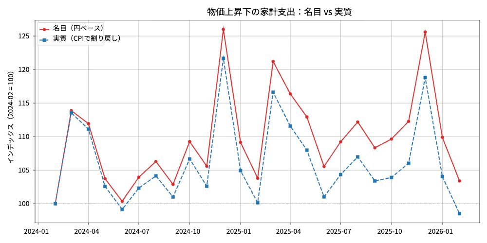
「名目では増えているのに実質では減っている」という事実が一目でわかります。

§7. まとめと注意点

今回の教訓：

統計 Excel は header=None で生読みして、iloc で抜き出すのが一番確実。
構造が謎なときは openpyxl で 1 セルずつ覗く。merged_cells.ranges を見れば罠の場所がわかる。
merged の残骸は '' か None になるので、ffill() で埋めればいい。
「年 + 月」が混ざった列は、無理にパースせず年だけ ffill して月を切り出す。

注意点：

統計資料は 改訂のたびに行・列がズレる ことがあります。iloc[14:, [3, 4, 8]] のようなハードコードは壊れる前提で。定期的にやるなら、ヘッダーの文字列を検索して列番号を探す関数を書くのが無難です。
今回は 4 列だけでしたが、CPI は 90 列以上あります。用途に応じて「品目名でマッチさせて列インデックスを動的に決める」処理が必要になるかもしれません。
fudebako はブラウザ完結なので社内分析にも使いやすいですが、/drive のファイルはブラウザを切り替えると消えます。大事なデータはローカルに保存しておきましょう。

動画化・転載歓迎

この記事の内容を YouTube 動画 / Podcast / 社内資料等に転載される際は、自由にお使いください。事前連絡は不要ですが、コメント欄や DM でお知らせいただけると今後の参考にさせていただきます。

You get articles that match your needs
You can efficiently read back useful information
You can use dark theme

What you can do with signing up