一言でいうと
Sanity Checks for Saliency Methodsの雑な再現実験をした話。
はじめに
LIME, Grad-CAM, SHAPなど、複雑な識別モデルの説明法がたびたび話題になり、日本語でも数々の素晴らしい記事が執筆されております。
本記事では、これらの手法の「不確かさ」を扱った論文であるSanity Checks for Saliency Methodsについて軽くまとめ、その再現実験をします。
Sanity Checks for Saliency Methods について
話題の説明法は、ヒートマップを用いて視覚的に識別の根拠を説明しています。
しかし、複雑なよく分からないモデルの根拠を説明しているため、真に求めるべきヒートマップを我々はうかがい知ることができません (知っているならばこれらの方法で説明する必要はありません)。
そのため、一部の手法の正当性は人間が視覚的に受ける印象で評価されていました。
この論文ではモデルのパラーメータ(重み)と視覚的な説明の関係を調べることで、一部の手法は正当性がないことを示しています。

上の図は、左上に示された鳥の画像に対して、Saliency Methodsと呼ばれる手法で説明した結果になります。
行ごとに異なる手法で説明しており、左から順に、学習済みのネットワークに対して説明したもの、そのネットワークのLogits層の重みをランダムな値に置き換えたネットワークに対して説明したもの、さらに入力に近い層の重みをランダム値に置き換えた・・・と続きます。
すなわち、一番右の結果は重みが全てランダムな意味のない識別器に対する説明になります。
意味のない識別器がなぜ鳥について説明できるのでしょうか?
一部の説明法はネットワークの重みとは関係のない、全く意味のない説明をしていたのではないでしょうか?
見た目で評価して大丈夫なのでしょうか?
そのような問いを投げかける論文です。
論文の詳細は関東・関西の論文読み会でそれぞれ紹介されているので、そちらもご覧下さい。
NeurIPS2018読み会@PFNで発表されたスライド
NIPS+読み会・関西 #7で発表されたスライド
実験
元論文には以下のように記述されているにもかかわらず、未だにgithubは更新されていないので再現実験をしました。
(last revised 28 Oct 2018)
All code to replicate our findings will be available here: https://goo.gl/hBmhDt
概要
全てGoogle Colaboratory上で実行することを想定しています。
識別モデルはTensorFlow Hubから学習済みのものをダウンロードして使い、Saliencyライブラリで説明(可視化)します。
実験環境
2019年5月27日にGoogle Colaboratoryで実行可能であることを確認しています。
Googleドライブ上の任意の位置に説明対象の画像を配置しているものとします。
Notebook
まず、説明(可視化)法のライブラリであるSaliencyをインストールします。
ライブラリについてはpypipの公式
https://pypi.org/project/saliency/
またはgithubレポジトリをご確認ください。
https://github.com/PAIR-code/saliency
!pip install saliency
次に、ダウンロードした画像を読み込むためにGoogle Driveをマウントします。
Googleアカウントでログインし、認証コードを入力してください
from google.colab import drive
drive.mount('/content/drive')
TensorFlow Hubから学習済みのInception v3を読み込みます。
TensorFlow Hub上にある学習済みモデルの一覧はこちらから確認できます。
import tensorflow_hub as hub

module = hub.Module("https://tfhub.dev/google/imagenet/inception_v3/classification/3")
TensorFlow Hubの使い方(折りたたみ)
module.get_signature_names()でモデルの識別用途(シグネイチャ)が表示できます。
後に出てくるget_〇〇()メソッドの引数に用いることがあるので、確認してください。
module.get_signature_names()
['image_feature_vector',
'image_classification_with_bn_hparams',
'image_feature_vector_with_bn_hparams',
'default',
'image_classification']
画像の特徴量の抽出と識別の2つのシグネイチャがあることがわかります。
_with_bn_hparamsはバッチ正規化の指数移動平均のハイパーパラメータを設定する場合に使います。
詳細は公式をご覧下さい。
次に、moduleへの入力を確認します。
get_input_info_dict()メソッドで入力すべきテンソルに関する情報が得られます。
module.get_input_info_dict()
{'images': <hub.ParsedTensorInfo shape=(?, ?, ?, 3) dtype=float32 is_sparse=False>}
入力層は"images"という名前で任意長のカラー画像を入力として用いることがわかります。
get_output_info_dict(signature='XXX")は取得できる(内部も含めた)出力の情報が得られます。
for outputName in sorted(module.get_output_info_dict(signature='image_feature_vector').items()):
  print(outputName)
('InceptionV3/Conv2d_1a_3x3', <hub.ParsedTensorInfo shape=(?, ?, ?, 32) dtype=float32 is_sparse=False>)
('InceptionV3/Conv2d_2a_3x3', <hub.ParsedTensorInfo shape=(?, ?, ?, 32) dtype=float32 is_sparse=False>)
('InceptionV3/Conv2d_2b_3x3', <hub.ParsedTensorInfo shape=(?, ?, ?, 64) dtype=float32 is_sparse=False>)
...
この名前は、任意の層の出力を取り出す場合に用いるので必ず確認してください。
次は変数の名前を取り出す方法です。
module.variablesで表示でき、それぞれの変数は名前やshapeを持っています。
for elem in module.variables:
  print(elem.name,":",elem.shape)
module/InceptionV3/Conv2d_1a_3x3/BatchNorm/beta:0 : (32,)
module/InceptionV3/Conv2d_1a_3x3/BatchNorm/moving_mean:0 : (32,)
module/InceptionV3/Conv2d_1a_3x3/BatchNorm/moving_variance:0 : (32,)
module/InceptionV3/Conv2d_1a_3x3/weights:0 : (3, 3, 3, 32)
module/InceptionV3/Conv2d_2a_3x3/BatchNorm/beta:0 : (32,)
...
メンバ変数やメソッドの説明はここで終わりです。
必要なライブラリをインポートします。
また、入力のplaceholderは準備する必要があるので、サイズは299x299として定義します (任意の値にしてください)。
そしてそのplaceholderをmoduleに引数として与え、シグネイチャは"image_classification"とします。
任意の層の出力は辞書型のキー (確認方法は折りたたみ内の説明) を与えることで取得できます。
from PIL import Image
import numpy as np
import matplotlib.pyplot as plt

import tensorflow as tf

# Input Placeholder
images = tf.placeholder(tf.float32, (None, 299, 299, 3))

# Set Placeholder & Set module type
outputs = module(dict(images=images), signature="image_classification", as_dict=True)

y_pred = outputs['InceptionV3/Predictions']
y_logits = outputs['InceptionV3/Logits']
入力をGoogle Driveから取ってきます。ここではシマウマの画像を使用します。
そして、先ほど指定したサイズに画像をリサイズし、前処理として画像の値を0~1にします。
必要な前処理の方法は基本的に公式に書いてあります (たまになかったりしますが、画像では基本的に画像の値を0~1にすればOKです)。
img = Image.open("./drive/My Drive/Colab Notebooks/images/zebra.jpg")
img_resize = img.resize((299, 299))
img_resize = np.reshape(img_resize,[1,299,299,3])/255
Sessionを用意して初期化します。
init_ops = [tf.global_variables_initializer(), tf.tables_initializer()]

session = tf.Session()
session.run(init_ops)
シマウマ画像を入力し、そのときの出力を確認します。
ラベルの番号については公式で確認できます。
シマウマは341番です。
pred = session.run(y_pred,feed_dict={images:img_resize})
print(np.shape(pred))
print(np.argmax(pred))
print(pred[0][341])
(1, 1001)
341
0.98961556
正しく識別されています。
次に可視化ライブラリのインスタンスを生成します。
ここで用いる説明法は勾配をもとに計算しているため、入力と出力、さらにグラフとセッションを与える必要があります。
また、シマウマらしい箇所に関しての説明が必要なため、出力の341番目のニューロンを指定しています。
クラスを動的に変更させたい場合はplaceholderを用いればOKです。
Occulusionは計算コストが高く、時間がかかるためコメントアウトしています。
pipで入るsaliencyはバージョンが古く、Grad-CAMはないので省略しています。
(Grad-CAMを使いたいならば、自身でgithubからクローンしたパッケージを使って下さい)
from saliency import GuidedBackprop
from saliency import IntegratedGradients
# from saliency import Occlusion
from saliency import GradientSaliency

guided_backprop_saliency = GuidedBackprop(tf.get_default_graph(), session, y_logits[0][341], images)
integrated_gradients_saliency = IntegratedGradients(tf.get_default_graph(), session, y_logits[0][341], images)
# occulusion_saliency = Occlusion(tf.get_default_graph(), session, y_logits[0][341], images)
gradient_saliency = GradientSaliency(tf.get_default_graph(), session, y_logits[0][341], images)
次に、順に重みを"破壊"するために破壊対象の重みを示したリストを用意します。
重みの破壊では、ランダムなテンソルを生成して置き換えるためにshapeと変数名が必要なので取得します。
target_layers = ["Logits","Mixed_7c","Mixed_7b","Mixed_7a","Mixed_6e","Mixed_6d","Mixed_6c",
                 "Mixed_6b","Mixed_6a","Mixed_5d","Mixed_5c","Mixed_5b","Conv2d_4a_3x3",
                 "Conv2d_3b_1x1","Conv2d_2b_3x3","Conv2d_2a_3x3","Conv2d_1a_3x3"]

target_shapes = []
target_names = []

for layer_name in target_layers:
  for module_variable in module.variables:
    if layer_name in module_variable.name:
      if "weight" in module_variable.name:
        target_shapes.append(module_variable.get_shape().as_list())
        target_names.append(module_variable.name)
        break
print(target_names)
print(target_shapes)
['module/InceptionV3/Logits/Conv2d_1c_1x1/weights:0', 'module/InceptionV3/Mixed_7c/Branch_0/Conv2d_0a_1x1/weights:0', 'module/InceptionV3/Mixed_7b/Branch_0/Conv2d_0a_1x1/weights:0', 'module/InceptionV3/Mixed_7a/Branch_0/Conv2d_0a_1x1/weights:0', 'module/InceptionV3/Mixed_6e/Branch_0/Conv2d_0a_1x1/weights:0', 'module/InceptionV3/Mixed_6d/Branch_0/Conv2d_0a_1x1/weights:0', 'module/InceptionV3/Mixed_6c/Branch_0/Conv2d_0a_1x1/weights:0', ...]
[[1, 1, 2048, 1001], [1, 1, 2048, 320], [1, 1, 1280, 320], [1, 1, 768, 192], [1, 1, 768, 192], [1, 1, 768, 192], [1, 1, 768, 192], [1, 1, 768, 192], [3, 3, 288, 384], [1, 1, 288, 64], [1, 1, 256, 64], [1, 1, 192, 64], [3, 3, 80, 192], [1, 1, 64, 80], [3, 3, 32, 64], [3, 3, 32, 32], [3, 3, 3, 32]]
描画の設定と、描画のための関数を用意します。
from pylab import rcParams
rcParams["figure.figsize"] = 15,15

def plot_attribution(attribution, index, name, threshold=99):
  plt.subplot(1,6,index)
  plt.axis("off")
  plt.title(name)
  MAX = np.percentile(attribution,threshold)
  plt.imshow(attribution,cmap=plt.cm.coolwarm,vmin=-MAX,vmax=MAX)
最後に、順次重みをランダム値に置き換えながら説明(可視化)していきます。
for i in range(len(target_shapes)+1):
  # 識別結果の確認
  pred = session.run(y_pred,feed_dict={images:img_resize})
  print("Predicted Label:",np.argmax(pred), " Zebra:",pred[0][341])

  # 説明(可視化)対象の画像の表示
  plt.subplot(1,6,1)
  plt.axis("off")
  plt.title("Image")
  plt.imshow(img_resize[0])

  # 各々の説明法の実行と結果の描画
  plot_attribution(gradient_saliency.GetMask(img_resize[0]).sum(axis=2),
                   2,
                   "Vanilla Grad.")
  plot_attribution(gradient_saliency.GetSmoothedMask(img_resize[0],magnitude=False).sum(axis=2),
                   3,
                   "Vanilla Grad. with SG")

  plot_attribution(np.sum(gradient_saliency.GetMask(img_resize[0]) * img_resize[0],axis=2),
                   4,
                   "Grad. x Input")

  plot_attribution(guided_backprop_saliency.GetMask(img_resize[0]).sum(axis=2),
                   5,
                   "GBP")

  plot_attribution(integrated_gradients_saliency.GetMask(img_resize[0]).sum(axis=2),
                   6,
                   "IG")

  # 描画または保存
  #plt.show()
  plt.savefig("./drive/My Drive/Colab Notebooks/Zebra4_"+str(i)+".png",bbox_inches="tight")
  plt.clf()

  # 最後の1ループは重みを破壊しないので除外
  if(i == len(target_shapes)):
    continue

  # 重みの破壊
  session.run(tf.assign(module.variable_map[target_names[i][7:-2]],  # 'module/XXX:0の不要な部分の削除
                        np.random.uniform(-1,1,target_shapes[i])))
  print("Randomized:",target_names[i][7:-2])
Predicted Label: 341 Zebra: 0.98961556
Randomized: InceptionV3/Logits/Conv2d_1c_1x1/weights
Predicted Label: 187 Zebra: 3.0443883e-17
Randomized: InceptionV3/Mixed_7c/Branch_0/Conv2d_0a_1x1/weights
Predicted Label: 906 Zebra: 0.0
Randomized: InceptionV3/Mixed_7b/Branch_0/Conv2d_0a_1x1/weights
Predicted Label: 559 Zebra: 0.0
Randomized: InceptionV3/Mixed_7a/Branch_0/Conv2d_0a_1x1/weights
Predicted Label: 559 Zebra: 0.0
Randomized: InceptionV3/Mixed_6e/Branch_0/Conv2d_0a_1x1/weights
Predicted Label: 966 Zebra: 0.0
Randomized: InceptionV3/Mixed_6d/Branch_0/Conv2d_0a_1x1/weights
Predicted Label: 559 Zebra: 0.0
Randomized: InceptionV3/Mixed_6c/Branch_0/Conv2d_0a_1x1/weights
Predicted Label: 559 Zebra: 0.0
Randomized: InceptionV3/Mixed_6b/Branch_0/Conv2d_0a_1x1/weights
Predicted Label: 500 Zebra: 0.0
Randomized: InceptionV3/Mixed_6a/Branch_0/Conv2d_1a_1x1/weights
Predicted Label: 500 Zebra: 0.0
Randomized: InceptionV3/Mixed_5d/Branch_0/Conv2d_0a_1x1/weights
Predicted Label: 500 Zebra: 0.0
Randomized: InceptionV3/Mixed_5c/Branch_0/Conv2d_0a_1x1/weights
Predicted Label: 559 Zebra: 0.0
Randomized: InceptionV3/Mixed_5b/Branch_0/Conv2d_0a_1x1/weights
Predicted Label: 500 Zebra: 0.0
Randomized: InceptionV3/Conv2d_4a_3x3/weights
Predicted Label: 966 Zebra: 0.0
Randomized: InceptionV3/Conv2d_3b_1x1/weights
Predicted Label: 469 Zebra: 0.0
Randomized: InceptionV3/Conv2d_2b_3x3/weights
Predicted Label: 469 Zebra: 0.0
Randomized: InceptionV3/Conv2d_2a_3x3/weights
Predicted Label: 469 Zebra: 0.0
Randomized: InceptionV3/Conv2d_1a_3x3/weights
Predicted Label: 469 Zebra: 0.0
結果画像
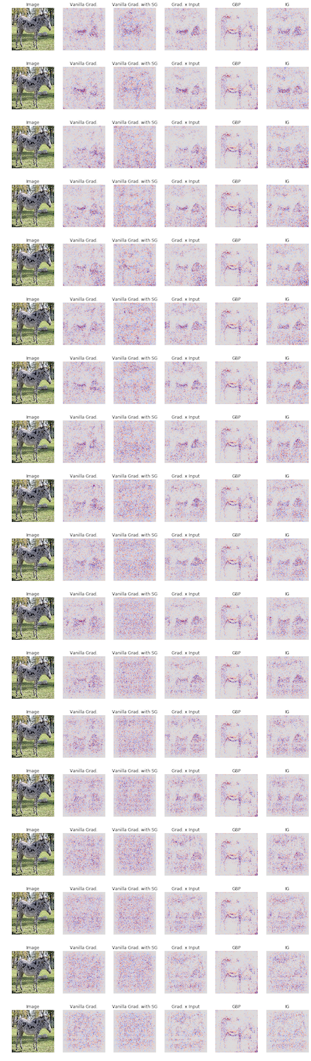
Guided Back-Propagationはモデルのパラメータと無関係な振る舞いをしていることが確認できました。
GBPは使わないようにしましょう!
おわりに
いかがでしたか?
識別モデルをMobileNetに変更する、俺が学習した最強の識別器でやってみる、他の説明法もためしてみる。など皆様も色々と実験してみて下さい。
他の説明法は以下のライブラリを使えばすぐに実装でいます。
https://github.com/marcoancona/DeepExplain
Colab上で実行できるのでPCの電気代以外ほぼ無料です。
PR・マサカリなど、なんでもぶん投げて下さい。お待ちしております。