はじめに
本記事はAdvent Calender「数値解析」の記事になります。最近、Rustで弾性体の二次元有限要素法プログラムを実装しています。本記事ではその振り返りをしたいと思います。
なぜRustなのか
Rustにした理由は単純にパフォーマンスを求めたかったからです。数値解析の実装でまず挙がるのはPythonかもしれませんが、Pythonで記述してもパフォーマンスの低さから後で使う気にはならない気がします。やはり作ったものは使いたいですよね。
C++と悩みましたが、友人のプログラマに話を聞いたところ「Rust一択!」と言われたのでRustにしました。このあたりは色々な意見があるかもしれませんが。
連続体の支配方程式
連続体の支配方程式をおさらいします。支配方程式は以下の3つの式からなります。
-
つり合い方程式(equilibrium condition)
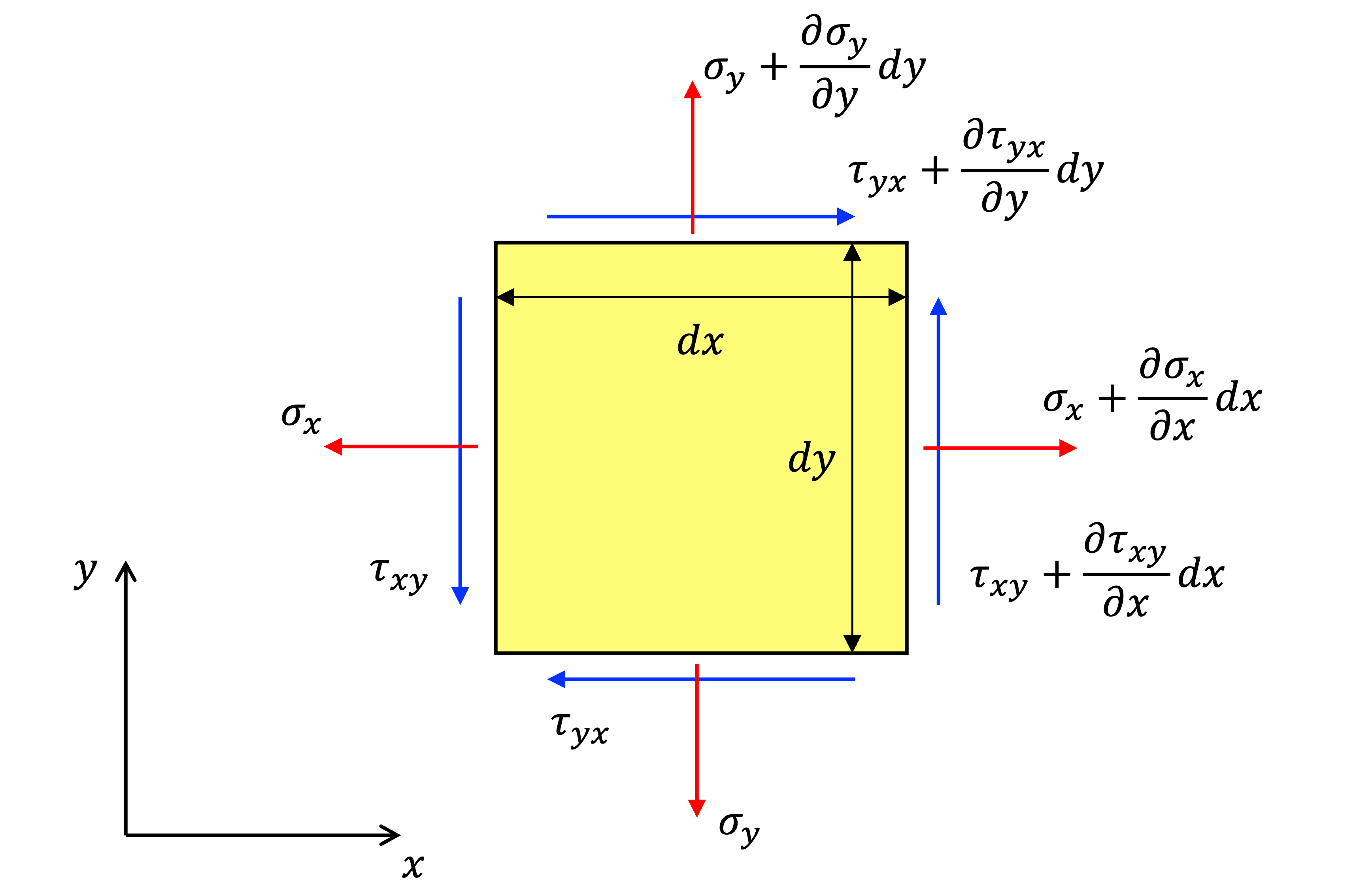
上図のような二次元微小変形要素があるとします。σが垂直応力τがせん断応力です。ここで、x軸方向のモーメントを考えると、
$$
\left(σ_x + \frac{\partial σ_x}{\partial x} dx \right)dy - σ_x dy + \left(τ_{yx} + \frac{\partial τ_{yx}}{\partial x} dx \right) dy - τ_{yx} dy + X dx dy = 0
$$
$$
\frac{\partial σ_x}{\partial x} + \frac{\partial τ_{xy}}{\partial x} + X = 0 \tag{1}
$$となります。ここで、Xは重力のような物体力を表しています。
同じようにy軸方向のモーメントを考えると、次式が得られます。$$
\left(σ_y + \frac{\partial σ_y}{\partial y} dy \right)dx - σ_y dx + \left(τ_{xy} + \frac{\partial τ_{xy}}{\partial y} dy \right) dx - τ_{xy} dx + Y dx dy = 0
$$
$$
\frac{\partial σ_y}{\partial y} + \frac{\partial τ_{xy}}{\partial y} + Y = 0 \tag{2}
$$Yも同じく物体力を示しています。z軸(中心点)方向のモーメントを考えると$τ_{xy}=τ_{yx}$となるため、つり合い方程式は以下のように求められます。
$$
\begin{align}
&\frac{\partial σ_x}{\partial x} + \frac{\partial τ_{xy}}{\partial x} + X = 0
&\frac{\partial σ_y}{\partial y} + \frac{\partial τ_{xy}}{\partial y} + Y = 0 \tag{3}
\end{align}
$$ -
ひずみの適合条件式(compatibility condition)
垂直ひずみとせん断ひずみは以下のように定義されます。
$$
ε_x = \frac{\partial u}{\partial x} \
\quad ε_y = \frac{\partial v}{\partial y} \
\quad γ_{xy} = \frac{\partial u}{\partial y} + \frac{\partial v}{\partial x} \tag{4}
$$ここで、uはx方向の変位、vはy方向の変位を表します。式(4)だけでは解の唯一性がないため、制約条件が必要です。これを適合条件式といい、次式で表されます。
$$
\frac{\partial^2 ε_x}{\partial x^2} + \frac{\partial^2 ε_y}{\partial y^2} = \frac{\partial^2 γ_{xy}}{\partial x \partial y} \tag{5}
$$ -
構成式(constitutive equation)
構成式は応力とひずみの関係です。弾性体の構成式はおなじみフックの法則の拡張版で以下で表されます。$$
σ = D ε \tag{6}
$$Dは一次元の場合の弾性係数に相当するマトリクスで具体型は後述します。
有限要素法による解法
有限要素法は、対象を細かい要素に分割し各要素に重み付き残差法を用いる解析法になります。重み付き残差法としてはガラーキン法がよく用いられますがここでは割愛します。なお、これから先の解法は微小変形理論による等方線形弾性体を対象としたものです。
以下に有限要素法の具体形を示します。
応力ーひずみ関係
先程示した構成式の具体形を以下に示します。
\sigma = D \epsilon \tag{7}
\begin{pmatrix} \sigma_x \\ \sigma_y \\ \tau_{xy} \end{pmatrix} = \frac{E}{(1 - 2 \nu)(1 + \nu)} \begin{bmatrix} 1 & \nu & 0 \\ \nu & 1 & 0 \\ 0 & 0 & \frac{1 - 2 \nu}{\nu} \end{bmatrix} \begin{pmatrix} \epsilon_x \\ \epsilon_y \\ \gamma_{xy} \end{pmatrix} \tag{8}
ここで、$E$は弾性係数、$\nu$はポアソン比をしめしますここでは平面ひずみ条件(奥行き方向に無限大と仮定)としています。
境界条件式
境界条件は定義域の境界を規定するノイマン境界条件と外力等の値を直に与えるディリクレ境界条件があります。具体形は以下で表されます。
\begin{pmatrix} u \\ v \end{pmatrix} = \begin{pmatrix} \bar{u} \\ \bar{v} \end{pmatrix} \quad \rm{on} \quad \Gamma_u \tag{9}
\begin{bmatrix} n_x & 0 & n_y \\ 0 & n_y & n_x \end{bmatrix} \begin{pmatrix} \sigma_x \\ \sigma_y \\ \tau_xy \end{pmatrix} = \begin{pmatrix} \bar{t}_x \\ \bar{t}_y \end{pmatrix} \quad \rm{on} \quad \Gamma_t \tag{10}
支配方程式の弱形式化
先程示した支配方程式は強形式(局所形)であり、有限要素法で解く場合は弱形式(大域的なつり合い状態を記述する)にする必要があります。以下には支配方程式の弱形式化を示します。
まず、実変位から任意のずれ(仮想変位)$(\delta u, \delta v)$を導入し変位解の候補を次式のように表します。
\boldsymbol{w} = \begin{pmatrix} u + \delta u \\ v + \delta v\end{pmatrix} \tag{11}
次に、仮想変位を物体に作用させた際の内力と外力による仕事のつり合いを考えます。仮想変位とつり合い条件式の両辺との内積を取ることで得られる仕事量を領域全体で積分します。
\int_\Omega \{\delta u \quad \delta v \} \left(\begin{bmatrix} \frac{\partial}{\partial x} & 0 & \frac{\partial}{\partial y} \\ 0 & \frac{\partial}{\partial y} & \frac{\partial}{\partial x} \end{bmatrix} \begin{pmatrix} \sigma_x \\ \sigma_y \\ \tau_{xy} \end{pmatrix} + \begin{pmatrix} X \\ Y \end{pmatrix}\right) dV = 0 \tag{12}
上式には外表面$\Gamma_t$における内力と外力ベクトルのつり合いが考慮されていません。よって外表面のつり合い条件式を考慮できるようにGreenの定理を適用します。
\displaylines{
\int_\Gamma \{\delta u \quad \delta v \} \begin{bmatrix} n_x & 0 & n_y \\ 0 & n_y & n_x \end{bmatrix} \begin{pmatrix} \sigma_x \\ \sigma_y \\ \tau_xy \end{pmatrix} dS \\ - \int_\Omega \{\delta u \quad \delta v \} \begin{bmatrix} \frac{\partial}{\partial x} & 0 & \frac{\partial}{\partial y} \\ 0 & \frac{\partial}{\partial y} & \frac{\partial}{\partial x} \end{bmatrix} \begin{pmatrix} \sigma_x \\ \sigma_y \\ \tau_{xy} \end{pmatrix} dV + \int_\Omega \{\delta u \quad \delta v \} \begin{pmatrix} X \\ Y \end{pmatrix} dV = 0 \tag{13}
}
ノイマン境界条件を考慮すると次式が得られます。
\displaylines{
\int_\Omega \{\delta u \quad \delta v \} \begin{bmatrix} \frac{\partial}{\partial x} & 0 & \frac{\partial}{\partial y} \\ 0 & \frac{\partial}{\partial y} & \frac{\partial}{\partial x} \end{bmatrix} \begin{pmatrix} \sigma_x \\ \sigma_y \\ \tau_{xy} \end{pmatrix} dV \\ = \int_\Omega \{\delta u \quad \delta v \} \begin{pmatrix} X \\ Y \end{pmatrix} dV + \int_{\Gamma_t} \{\delta u \quad \delta v \} \begin{pmatrix} \bar{t}_x \\ \bar{t}_y \end{pmatrix} dS \tag{14}
}
上式を系に作用する仮想的な仕事のつり合いを考慮した弱形式であり、仮想仕事の原理と呼びます。
空間の離散化
前節の弱形式を有限要素法で離散化します。ここでは、最も基本的かつ単純な4節点アイソパラメトリック要素を用います。アイソパラメトリック要素では、下図のように物理座標系$(x, y)$とは別の直行座標系$(a, b)$を導入します。
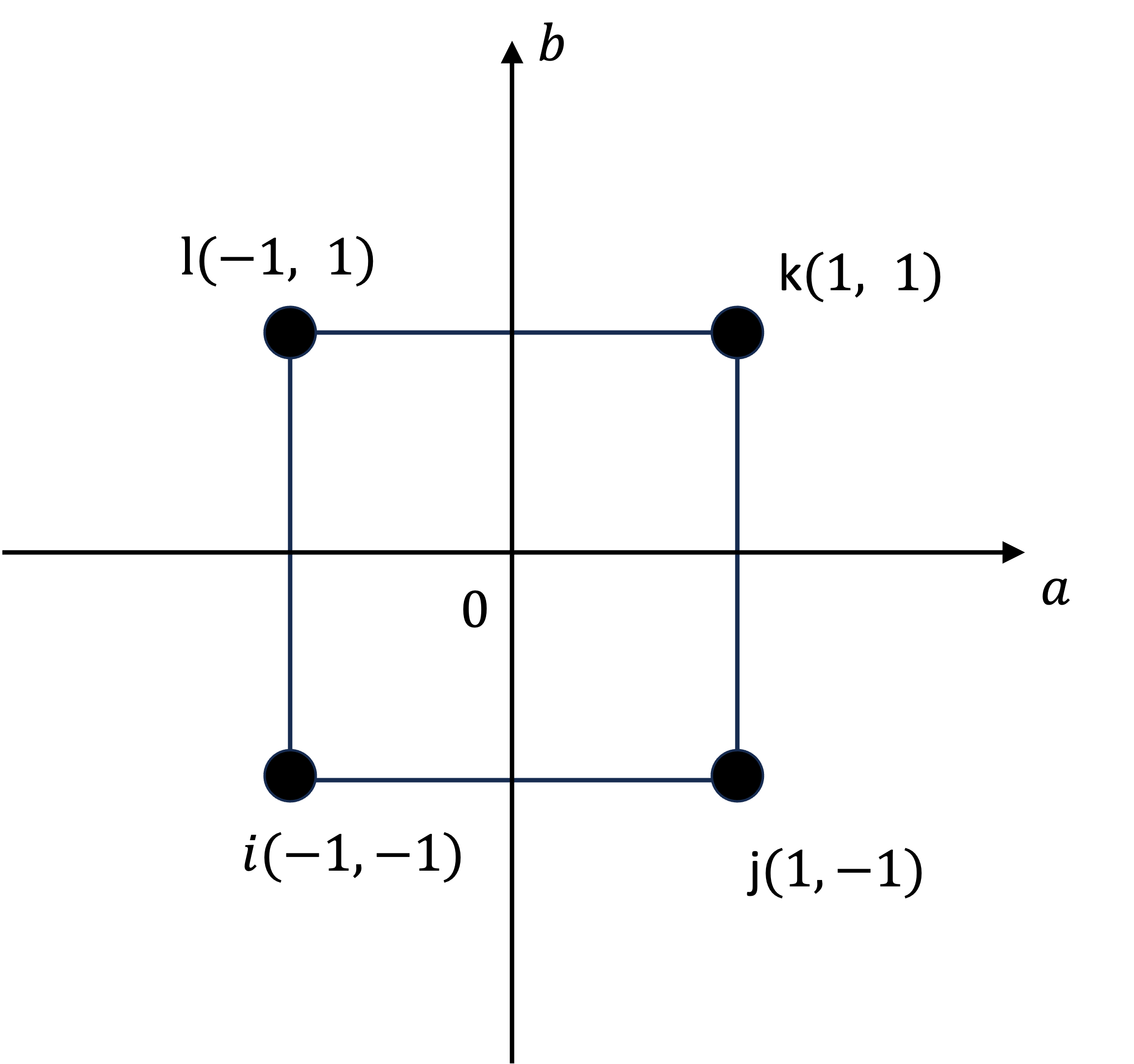
アイソパラメトリック要素を用いると、任意の点の変位は以下で表されます。
u(a, b) = N_i (a, b) u^e_i + N_j (a, b) u^e_j + N_k (a, b) u^e_k + N_l (a, b) u^e_l \tag{15}
v(a, b) = N_i (a, b) v^e_i + N_j (a, b) v^e_j + N_k (a, b) v^e_k + N_l (a, b) v^e_l \tag{16}
ここで、$N$は$(a, b)$を独立変数とする形状関数であり、以下で表されます。
\displaylines{
N_i = \frac{1}{4} (1 - a) (1 - b) \\
N_j = \frac{1}{4} (1 + a) (1 - b) \\
N_k = \frac{1}{4} (1 + a) (1 + b) \\
N_l = \frac{1}{4} (1 - a) (1 + b) \tag{17}
}
以上より、アイソパラメトリック要素を用いてひずみと応力が以下のように表されます。
\boldsymbol{\epsilon} = \partial \boldsymbol{u} = \partial \boldsymbol{N} \boldsymbol{d} = \boldsymbol{B} \boldsymbol{d} \quad \left(\boldsymbol{d} = \begin{pmatrix} \boldsymbol{u}^e \\ \boldsymbol{v}^e\end{pmatrix} \right) \tag{18}
ここで、$B$は次式で定義されるBマトリックスです。
\boldsymbol{B} = \partial \boldsymbol{N} = \begin{bmatrix} \frac{\partial N_i}{\partial x} & 0 & \frac{\partial N_j} {\partial x} & 0 & \frac{\partial N_k}{\partial x} & 0 & \frac{\partial N_l}{\partial x} & 0 \\ 0 & \frac{\partial N_i}{\partial y} & 0 & \frac{\partial N_j}{\partial y} & 0 & \frac{\partial N_k}{\partial y} & 0 & \frac{\partial N_l}{\partial y} \\ \frac{\partial N_i}{\partial x} & \frac{\partial N_i}{\partial y} & \frac{\partial N_j} {\partial x} & \frac{\partial N_j}{\partial y} & \frac{\partial N_k}{\partial x} & \frac{\partial N_k}{\partial y} & \frac{\partial N_l}{\partial x} & \frac{\partial N_l}{\partial y} \end{bmatrix} \tag{19}
内挿関数の微分はJacobi行列を用いて表すことができます。
\begin{bmatrix} J \end{bmatrix} = \begin{bmatrix} \frac{\partial x}{\partial a} & \frac{\partial y}{\partial a} \\ \frac{\partial x}{\partial b} & \frac{\partial y}{\partial b} \end{bmatrix} = \begin{bmatrix} J_{11} & J_{12} \\ J_{21} & J_{22} \end{bmatrix} \tag{20}
\displaylines{
J_{11} = \frac{\partial N_i}{\partial a} y_i + \frac{\partial N_j}{\partial a} y_j + \frac{\partial N_k}{\partial a} y_k + \frac{\partial N_l}{\partial a} y_l \\
J_{12} = \frac{\partial N_i}{\partial a} x_i + \frac{\partial N_j}{\partial a} x_j + \frac{\partial N_k}{\partial a} x_k + \frac{\partial N_l}{\partial a} x_l \\
J_{21} = \frac{\partial N_i}{\partial b} x_i + \frac{\partial N_j}{\partial b} x_j + \frac{\partial N_k}{\partial b} x_k + \frac{\partial N_l}{\partial b} x_l \\
J_{22} = \frac{\partial N_i}{\partial b} y_i + \frac{\partial N_j}{\partial b} y_j + \frac{\partial N_k}{\partial b} y_k + \frac{\partial N_l}{\partial b} y_l \tag{21}
}
変位の近似(式(15)(16))にとその変分、およびひずみの近似式(式(18))とその変分を要素の弱形式に導入すると、要素剛性方程式が得られます。
\boldsymbol{K}_e = \int_{\Omega_e} \boldsymbol{B}^T \boldsymbol{D} \boldsymbol{B} dV \tag{22}
ガウス積分
有限要素法では、数値積分法としてガウス積分が用いられます。積分点を4点とすると、以下のようにa, bの値と重みHが求まり、その総和が積分の近似値となります。
{\begin{align}
& i  & j & &  a              &&b              & & H              & & kk \\
& 1  & 1 & & -\frac{1}{\sqrt{3}}  & & -\frac{1}{\sqrt{3}}  & & 1.0  & & 1  \\\
& 1  & 2 & & \frac{1}{\sqrt{3}}  & & -\frac{1}{\sqrt{3}}  & & 1.0  & & 2  \\\
& 2  & 1 & & \frac{1}{\sqrt{3}}  & & \frac{1}{\sqrt{3}}  & & 1.0  & & 3  \\\
& 2  & 2 & & -\frac{1}{\sqrt{3}}  & & \frac{1}{\sqrt{3}}  & & 1.0  & & 4
\end{align}
}
ガウス積分を用いると、式(22)の要素剛性方程式は以下のように計算できます。
\boldsymbol{K}_e = \sum_{i=1}^2 \sum_{j=1}^2 \boldsymbol{B}^T(a_i, b_j) \boldsymbol{D} \boldsymbol{B}(a_i, b_j) |J(a_i, b_j)| \tag{23}
全体剛性方程式の組み立て
すべての要素$\Omega_e$に対して要素剛性方程式を求め、それらを節点の結合情報を参照してアセンブリすることで全体系の剛性方程式を求めることができます。
\boldsymbol{K} \boldsymbol{d} = \boldsymbol{F} \tag{24}
あとは全体剛性方程式を解くことで変位が求まり、変位からひずみ、応力を求めることができます。
全体剛性方程式を解くには何らかの連立方程式の解法が必要です。
Rustによる実装
Rustを用いてこれまで示した有限要素法を実装してみます。行列計算にはnalgebraというライブラリを用います。
(1)節点数、自由度の定義
const NODE_NUM: usize = 4;
const NODE_DOF: usize = 2;
(2)弾性体のDマトリクス情報を持つオブジェクト
struct Elastic {
    young: f64,
    poisson: f64,
}

impl Elastic {
    fn make_dematrix(&self) -> na::Matrix3<f64> {
        let tmp: f64 = self.young / (1.0 + self.poisson) / (1.0 - 2.0 * self.poisson);
        let mut mat_d = na::Matrix3::<f64>::zeros();
        mat_d[(0, 0)] = 1.0 - self.poisson;
        mat_d[(0, 1)] = self.poisson;
        mat_d[(1, 0)] = self.poisson;
        mat_d[(1, 1)] = 1.0 - self.poisson;
        mat_d[(2, 2)] = 0.5 * (1.0 - 2.0 * self.poisson);
        mat_d *= tmp;
        return mat_d;
    }
}
(3)2次元4節点の全体剛性マトリクスの情報を持つオブジェクト
struct C2D4 {
    nodes: na::Matrix2xX<f64>,
    elements: na::Matrix6xX<usize>,
    materials: na::Matrix3xX<f64>,
}

impl C2D4 {
    //全体剛性マトリクスの計算
    fn make_global_kmatrix(&self) -> na::DMatrix<f64> {
        let mut mat_k =
            na::DMatrix::<f64>::zeros(NODE_DOF * self.nodes.ncols(), NODE_DOF * self.nodes.ncols());
        let mut ir = na::DVector::<usize>::zeros(NODE_DOF * NODE_NUM);

        for ele in 0..self.elements.ncols() {
            let mat_ke = self.make_kematrix(ele);
            let i = self.elements[(1, ele)];
            let j = self.elements[(2, ele)];
            let k = self.elements[(3, ele)];
            let l = self.elements[(4, ele)];
            //println!("{}", i);
            ir[7] = 2 * l - 1;
            ir[6] = ir[7] - 1;
            ir[5] = 2 * k - 1;
            ir[4] = ir[5] - 1;
            ir[3] = 2 * j - 1;
            ir[2] = ir[3] - 1;
            ir[1] = 2 * i - 1;
            ir[0] = ir[1] - 1;

            for ii in 0..(NODE_DOF * NODE_NUM) {
                let it = ir[ii];

                for jj in 0..(NODE_DOF * NODE_NUM) {
                    let jt = ir[jj];
                    mat_k[(it, jt)] = mat_k[(it, jt)] + mat_ke[(ii, jj)];
                }
            }
        }

        return mat_k;
    }

    //要素剛性マトリクスの計算
    fn make_kematrix(&self, ele: usize) -> DMatrix<f64> {
        let mut mat_ke = DMatrix::<f64>::zeros(NODE_DOF * NODE_NUM, NODE_DOF * NODE_NUM);
        let m = self.elements[(5, ele)] - 1;
        //println!("{}", m);
        let elastic = Elastic {
            young: self.materials[(1, m)],
            poisson: self.materials[(2, m)],
        };
        let mat_d = elastic.make_dematrix();
        //println!("{}", mat_d);

        for ii in 0..NODE_NUM {
            let mat_j = self.make_jmatrix(ele, ii);
            let mat_b = self.make_bmatrix(ii, mat_j);
            //println!("{}", mat_b);
            mat_ke += mat_b.transpose() * mat_d * mat_b * mat_j.determinant();
        }

        return mat_ke;
    }

    //ヤコビ行列の計算
    fn make_jmatrix(&self, ele: usize, ii: usize) -> na::Matrix2<f64> {
        let gauss = self.gauss_point(ii);
        let dndab = self.make_dndab(gauss.0, gauss.1);
        let i = self.elements[(1, ele)] - 1;
        let j = self.elements[(2, ele)] - 1;
        let k = self.elements[(3, ele)] - 1;
        let l = self.elements[(4, ele)] - 1;
        let mat_xiyi = na::Matrix4x2::new(
            self.nodes[(0, i)],
            self.nodes[(1, i)],
            self.nodes[(0, j)],
            self.nodes[(1, j)],
            self.nodes[(0, k)],
            self.nodes[(1, k)],
            self.nodes[(0, l)],
            self.nodes[(1, l)],
        );
        //println!("{}", mat_xiyi);
        let mat_j = &dndab * &mat_xiyi;
        return mat_j;
    }

    //Bマトリックスの計算
    fn make_bmatrix(&self, ii: usize, mat_j: na::Matrix2<f64>) -> na::SMatrix<f64, 3, 8> {
        let gauss = self.gauss_point(ii);
        let dndab = self.make_dndab(gauss.0, gauss.1);
        let dndxy = mat_j.transpose() * dndab;
        let mut mat_b = na::SMatrix::<f64, 3, 8>::zeros();
        mat_b[(0, 0)] = dndxy[(0, 0)];
        mat_b[(0, 2)] = dndxy[(0, 1)];
        mat_b[(0, 4)] = dndxy[(0, 2)];
        mat_b[(0, 6)] = dndxy[(0, 3)];
        mat_b[(1, 1)] = dndxy[(1, 0)];
        mat_b[(1, 3)] = dndxy[(1, 1)];
        mat_b[(1, 5)] = dndxy[(1, 2)];
        mat_b[(1, 7)] = dndxy[(1, 3)];
        mat_b[(2, 0)] = dndxy[(1, 0)];
        mat_b[(2, 1)] = dndxy[(0, 0)];
        mat_b[(2, 2)] = dndxy[(1, 1)];
        mat_b[(2, 3)] = dndxy[(0, 1)];
        mat_b[(2, 4)] = dndxy[(1, 2)];
        mat_b[(2, 5)] = dndxy[(0, 2)];
        mat_b[(2, 6)] = dndxy[(1, 3)];
        mat_b[(2, 7)] = dndxy[(0, 3)];
        return mat_b;
    }

    //ガウス積分
    fn gauss_point(&self, ii: usize) -> (f64, f64) {
        let tmp = (1.0 / 3.0 as f64).sqrt();

        if ii == 1 {
            let ai = (-1.0) * tmp;
            let bi = (-1.0) * tmp;
            return (ai, bi);
        } else if ii == 2 {
            let ai = tmp;
            let bi = (-1.0) * tmp;
            return (ai, bi);
        } else if ii == 3 {
            let ai = tmp;
            let bi = tmp;
            return (ai, bi);
        } else {
            let ai = (-1.0) * tmp;
            let bi = tmp;
            return (ai, bi);
        }
    }

    //形状関数の微分
    fn make_dndab(&self, ai: f64, bi: f64) -> na::Matrix2x4<f64> {
        let dn1da = -0.25 * (1.0 - bi);
        let dn2da = 0.25 * (1.0 - bi);
        let dn3da = 0.25 * (1.0 + bi);
        let dn4da = -0.25 * (1.0 + bi);
        let dn1db = -0.25 * (1.0 - ai);
        let dn2db = -0.25 * (1.0 + ai);
        let dn3db = 0.25 * (1.0 + ai);
        let dn4db = 0.25 * (1.0 - ai);
        let dndab = na::Matrix2x4::new(dn1da, dn2da, dn3da, dn4da, dn1db, dn2db, dn3db, dn4db);
        return dndab;
    }
}
(4)境界条件を設定するオブジェクト
struct Boundary2d {
    nodes: na::Matrix2xX<f64>,
    total_time: na::DVector<f64>,
    delta_time: na::DVector<f64>,
    force_node: na::DVector<usize>,
    force_node_xy: na::DMatrix<f64>,
    disp_node_no: na::DMatrix<usize>,
    disp_node_xy: na::DMatrix<f64>,
}

impl Boundary2d {
    fn make_force_vector(&self, ii: usize, jj: usize) -> na::DVector<f64> {
        let mut vec_f = na::DVector::zeros(NODE_DOF * self.nodes.ncols());
        let tmp = NODE_DOF * self.nodes.ncols();

        for i in 0..tmp {
            if self.force_node[ii] > 0 {
                vec_f[i] = self.force_node_xy[(ii, i)] / self.total_time[ii] * self.delta_time[ii];
            } else {
                vec_f[i] = 0.0;
            }
        }

        return vec_f;
    }

    fn mat_boundary_setting(
        &self,
        mat_k: na::DMatrix<f64>,
        vec_f: DVector<f64>,
    ) -> (na::DMatrix<f64>, na::DVector<f64>) {
        let mut mat_k_c = mat_k.clone();
        let mut vec_f_c = vec_f.clone();

        for ii in 0..self.nodes.ncols() {
            for jj in 0..NODE_DOF {
                if self.disp_node_no[(jj, ii)] == 1 {
                    let iz = ii * NODE_DOF + jj;
                    vec_f_c[iz] = 0.0;
                }
            }
        }

        for ii in 0..self.nodes.ncols() {
            for jj in 0..NODE_DOF {
                if self.disp_node_no[(jj, ii)] == 1 {
                    let iz = ii * NODE_DOF + jj;
                    let vecx = mat_k.column(iz);
                    vec_f_c -= self.disp_node_xy[(jj, ii)] * vecx;

                    for kk in 0..self.nodes.ncols() * NODE_DOF {
                        mat_k_c[(kk, iz)] = 0.0;
                    }

                    mat_k_c[(iz, iz)] = 1.0;
                }
            }
        }
        return (mat_k_c, vec_f_c);
    }

    fn disp_boundary_setting(&self, disp_tri: DVector<f64>) -> na::DVector<f64> {
        let mut disp_tri_c = disp_tri.clone();

        for ii in 0..self.nodes.ncols() {
            for jj in 0..NODE_DOF {
                if self.disp_node_no[(jj, ii)] == 1 {
                    let iz = ii * NODE_DOF + jj;
                    disp_tri_c[iz] = self.disp_node_xy[(jj, ii)];
                }
            }
        }

        return disp_tri_c;
    }
}
(5)入力データの読み込み
fn input_data(
    filename: &str,
) -> (
    na::Matrix2xX<f64>,
    na::Matrix6xX<usize>,
    na::Matrix3xX<f64>,
    na::DMatrix<usize>,
    na::DMatrix<f64>,
    usize,
    na::DVector<f64>,
    na::DVector<f64>,
    na::DVector<usize>,
    na::DMatrix<f64>,
) {
    let file = std::fs::File::open(filename).unwrap();
    let reader = std::io::BufReader::new(file);
    let mut lines = reader.lines();
    let first_line = lines.next().unwrap().unwrap();
    let parts: Vec<&str> = first_line.split_whitespace().collect();
    let number_of_node: usize = parts[0].parse().unwrap();
    let number_of_element: usize = parts[1].parse().unwrap();
    let number_of_material: usize = parts[2].parse().unwrap();
    let number_of_pfix: usize = parts[3].parse().unwrap();
    let number_of_step: usize = parts[4].parse().unwrap();
    let mut nodes = na::Matrix2xX::zeros(number_of_node);

    //Nodes
    for i in 0..number_of_node {
        let line = lines.next().unwrap().unwrap();
        let parts: Vec<f64> = line
            .split_whitespace()
            .map(|s| s.parse().unwrap())
            .collect();
        //println!("{}, {}", parts[1], parts[2]);
        //let tmp = parts[0] as i32;
        nodes[(0, i)] = parts[1];
        nodes[(1, i)] = parts[2];
    }


    let mut elements = na::Matrix6xX::zeros(number_of_element);

    //Elements
    for i in 0..number_of_element {
        let line = lines.next().unwrap().unwrap();
        let parts: Vec<usize> = line
            .split_whitespace()
            .map(|s| s.parse().unwrap())
            .collect();
        elements[(0, i)] = parts[0];
        elements[(1, i)] = parts[1];
        elements[(2, i)] = parts[2];
        elements[(3, i)] = parts[3];
        elements[(4, i)] = parts[4];
        elements[(5, i)] = parts[5];
    }

    let mut materials = na::Matrix3xX::zeros(number_of_material);

    //Materials
    for i in 0..number_of_material {
        let line = lines.next().unwrap().unwrap();
        let parts: Vec<f64> = line
            .split_whitespace()
            .map(|s| s.parse().unwrap())
            .collect();
        materials[(0, i)] = parts[1];
        materials[(1, i)] = parts[2];
        materials[(2, i)] = parts[3];
    }

    let mut disp_node_no = na::DMatrix::zeros(NODE_DOF, number_of_node);
    let mut disp_node_xy = na::DMatrix::zeros(NODE_DOF, number_of_node);

    //Neunman boundary condition
    if number_of_pfix > 0 {
        for i in 0..number_of_pfix {
            let line = lines.next().unwrap().unwrap();
            let parts: Vec<f64> = line
                .split_whitespace()
                .map(|s| s.parse().unwrap())
                .collect();
            let tmp = parts[0] as usize;
            //println!("{}", tmp);
            disp_node_no[(0, tmp - 1)] = parts[1] as usize;
            disp_node_no[(1, tmp - 1)] = parts[2] as usize;
            disp_node_xy[(0, tmp - 1)] = parts[3];
            disp_node_xy[(1, tmp - 1)] = parts[4];
        }
    }

    //Analysis steps
    let mut total_time = na::DVector::zeros(number_of_step);
    let mut delta_time = na::DVector::zeros(number_of_step);
    let mut force = na::DVector::zeros(number_of_step);
    let mut force_node_no = na::DMatrix::zeros(number_of_step, number_of_node);
    let mut force_node_xy = na::DMatrix::zeros(number_of_step, number_of_node * NODE_DOF);

    for i in 0..number_of_step {
        let line = lines.next().unwrap().unwrap();
        let parts: Vec<f64> = line
            .split_whitespace()
            .map(|s| s.parse().unwrap())
            .collect();
        total_time[i] = parts[1];
        delta_time[i] = parts[2];
        force[i] = parts[3] as usize;

        //Dirichlet boundary condition
        if force[i] > 0 {
            for j in 0..force[i] {
                let line = lines.next().unwrap().unwrap();
                let parts: Vec<f64> = line
                    .split_whitespace()
                    .map(|s| s.parse().unwrap())
                    .collect();
                let tmp = parts[0] as usize;
                //println!("{}", tmp);
                force_node_no[(i, j)] = tmp;
                force_node_xy[(i, NODE_DOF * tmp - 2)] = parts[1];
                force_node_xy[(i, NODE_DOF * tmp - 1)] = parts[2];
            }
        }
    }
    return (
        nodes,
        elements,
        materials,
        disp_node_no,
        disp_node_xy,
        number_of_step,
        total_time,
        delta_time,
        force,
        force_node_xy,
    );
}
(5)FEMのメイン部分(連立方程式の計算まで)
fn fem() {
    //Read input data
    let inputdata = input_data("input/input.txt");
    let nodes = inputdata.0;
    let elements = inputdata.1;
    let materials = inputdata.2;
    let disp_node_no = inputdata.3;
    let disp_node_xy = inputdata.4;
    let number_of_step = inputdata.5;
    let total_time = inputdata.6;
    let delta_time = inputdata.7;
    let force_node = inputdata.8;
    let force_node_xy = inputdata.9;
    let matrix = C2D4 {
        nodes: nodes.clone(),
        elements: elements.clone(),
        materials: materials.clone(),
    };
    let boundary = Boundary2d {
        nodes: nodes.clone(),
        total_time: total_time.clone(),
        delta_time: delta_time.clone(),
        force_node: force_node.clone(),
        force_node_xy: force_node_xy.clone(),
        disp_node_no: disp_node_no.clone(),
        disp_node_xy: disp_node_xy.clone(),
    };

    //Analysis start
    for ii in 0..number_of_step {
        let time_step = (total_time[ii] / delta_time[ii]) as usize;

        for jj in 0..time_step {
            //Make global stiffness matrix
            let mat_k = matrix.make_global_kmatrix();
            //Make force vector
            let vec_f = boundary.make_force_vector(ii, jj);
            //Set boundary conditions
            let (mat_k_c, vec_f_c) = boundary.mat_boundary_setting(mat_k, vec_f);
            //Calcurate simultaneous equations using LU decomposition
            let tmp = mat_k_c.lu();
            let disp_tri = tmp.solve(&vec_f_c).expect("Linear resolution failed.");
            //Set boundary conditions
            let disp_tri_c = boundary.disp_boundary_setting(disp_tri);
        }
    }
}
おわりに
理論的部分を中心に有限要素法の実装までをまとめました。間違い、もっといい実装法がありましたらご連絡ください。
令和6年2月15日 ソースコード全体を公開しました。