前処理（特徴量エンジニアリング）

この記事の狙い・目的

機械学習を取り入れたAIシステムの構築は、
①データ分析→ ②データセット作成（前処理）→ ③モデルの構築・適用
というプロセスで行っていきます。
その際「前処理」の段階では、データ分析の考察を踏まえて、精度の高いデータセットが作れるよう様々な対応が必要となります。
このブログでは、「前処理（特徴量エンジニアリング）」の工程について初めから通して解説していきます。

プログラムの実行環境

Python3
MacBook pro（端末）
PyCharm（IDE）
Jupyter Notebook（Chrome）
Google スライド（Chrome）

データ確認

# データ取得
boston_df = pd.read_csv("./boston.csv", sep=',')

# データ確認
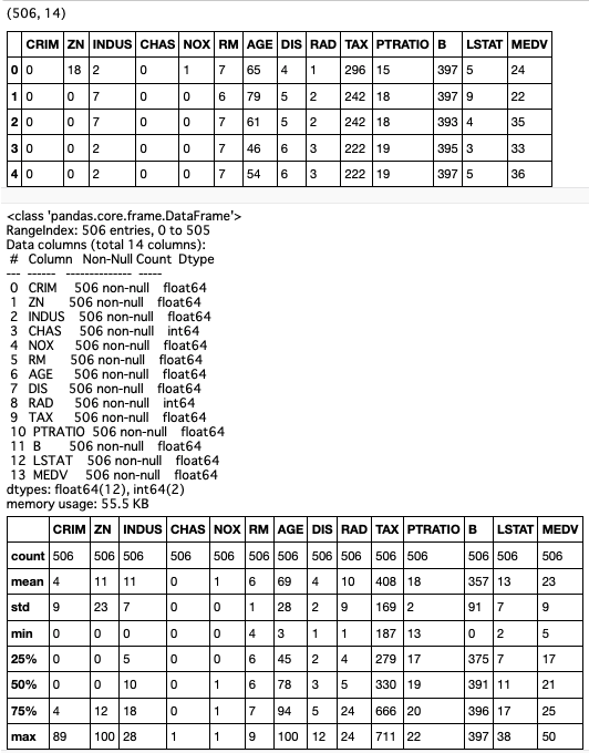
boston_df.shape
boston_df.head()
boston_df.info()
boston_df.describe()

精度評価

from sklearn.ensemble import RandomForestRegressor as RFR # ランダム・フォレスト（回帰）
from sklearn.model_selection import train_test_split # データ分割
from sklearn.metrics import r2_score, mean_squared_error, mean_absolute_error, mean_squared_log_error # 各評価指標

def learning(model, df):
    # データ分割
    X = df.drop('MEDV',axis=1)
    y = df['MEDV']
    X_train,X_test,y_train,y_test = train_test_split(X, y, test_size=0.2, random_state=42)

    # 学習、予測
    rfr_model = model
    rfr_model.fit(X_train, y_train)
    y_pred = rfr_model.predict(X_test).round(decimals=1)

    # 評価    
    print('決定係数（R2） = ', r2_score(y_test, y_pred).round(decimals=3))
    print('平均絶対誤差（MAE） = ', mean_absolute_error(y_test, y_pred).round(decimals=3))
    print('平均二乗誤差（MSE） = ', mean_squared_error(y_test, y_pred).round(decimals=3))
    print('対数平均二乗誤差（MSLE） = ', mean_squared_log_error(y_test, y_pred).round(decimals=3))
    print('平均二乗平方根誤差（RMSE） = ', np.sqrt(mean_squared_error(y_test, y_pred)).round(decimals=3))
    print('対数平方平均二乗誤差（RMSLE） = ', np.sqrt(mean_squared_log_error (y_test, y_pred)).round(decimals=3))

    return rfr_model, y_test, y_pred

# 実行
rfr_model, y_test, y_pred = learning(RFR(random_state=42), boston_df)

# 結果
# 決定係数（R2） =  0.892
# 平均絶対誤差（MAE） =  2.04
# 平均二乗誤差（MSE） =  7.902
# 対数平均二乗誤差（MSLE） =  0.02
# 平均二乗平方根誤差（RMSE） =  2.811
# 対数平方平均二乗誤差（RMSLE） =  0.142

非線形モデルでまずまずの評価

特徴量重要度

ランダム・フォレスト版

def rfr_importance(df):
    # データ分割
    X = df.drop(columns='MEDV', axis=1)
    y = df['MEDV']
    X_train, X_test, y_train, y_test = train_test_split(X, y, test_size=0.2, random_state=0)

    # モデリング
    clf_rf = RFR()
    clf_rf.fit(X_train, y_train)
    y_pred = clf_rf.predict(X_test)

    # 評価
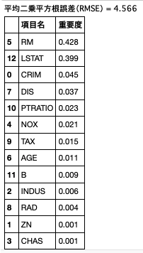
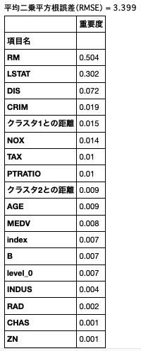
    print('平均二乗平方根誤差（RMSE） = {:>.3f}'.format(np.sqrt(mean_squared_error(y_test, y_pred))))

    # 重要度
    fimp = clf_rf.feature_importances_

    # データフレームに変換
    imp_df = pd.DataFrame()
    imp_df['項目名'] = df.columns[:-1]
    imp_df['重要度'] = fimp.round(decimals=3).astype(str)

    return imp_df

# 実行
imp_df = rfr_importance(boston_df)
imp_df.sort_values(by='重要度', ascending=False)

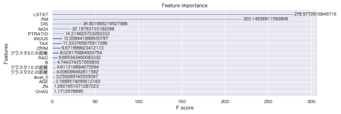
XGBoost版

import xgboost as xgb

def boost_importance(df):
    # データ分割
    X = df.drop(columns='MEDV', axis=1)
    y = df['MEDV']
    X_train, X_test, y_train, y_test = train_test_split(X, y, test_size=0.2, random_state=0)

    # パラメータ
    xgb_params = {"objective": "reg:linear", "eta": 0.1, "max_depth": 6, "silent": 1}
    num_rounds = 100

    # XGBoost用のデータセットの作成
    dtrain = xgb.DMatrix(X_train, label=y_train)

    # 学習
    gbdt = xgb.train(xgb_params, dtrain, num_rounds)

    # 重要度
    _, ax = plt.subplots(figsize=(12, 4))
    # パラメーター：gain 予測精度をどれだけ改善させたることができるできたか（平均値）
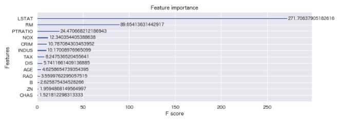
    xgb.plot_importance(gbdt, ax=ax, importance_type='gain')

# 実行
boost_importance(boston_df)

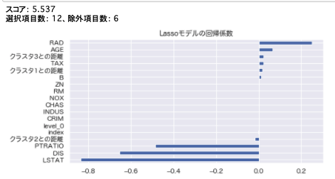
線形回帰モデル版

from sklearn.linear_model import Ridge, RidgeCV, ElasticNet, LassoCV, LassoLarsCV
from sklearn.model_selection import cross_val_score

def linear_importance(df):
    X = df.drop(columns='MEDV', axis=1)
    y = df['MEDV']
    X_train, X_test, y_train, y_test = train_test_split(X, y, test_size=0.2, random_state=0)

    def rmse_cv(model):
        rmse= np.sqrt(-cross_val_score(model, X_train, y_train, scoring="neg_mean_squared_error", cv = 5))
        return(rmse)

    # model_ridge = Ridge().fit(X_train, y_train)
    model_lasso = LassoCV().fit(X_train, y_train)
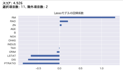
    print(f'スコア： {rmse_cv(model_lasso).mean().round(decimals=3)}')

    coef = pd.Series(model_lasso.coef_, index = X_train.columns)
    print("選択項目数： " + str(sum(coef != 0)) + "、除外項目数： " +  str(sum(coef == 0)))

    plt.figure(figsize=[8,4])
    imp_coef = coef.sort_values()
    imp_coef.plot(kind = "barh").grid()
    plt.title("Lassoモデルの回帰係数")

# 実行
linear_importance(boston_df)

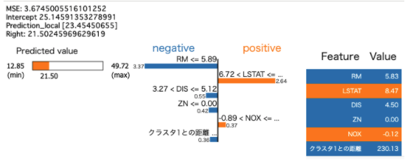
ランダム・フォレスト ＋ LIME版

import lime
import lime.lime_tabular

def explain_importance(df):
    # データ分割
    X = df.drop(columns='MEDV', axis=1)
    y = df['MEDV']
    X_train, X_test, y_train, y_test = train_test_split(X, y, test_size = 0.3, random_state = 0)

    # ランダム・フォレスト（回帰）
    model = RFR(max_depth=6, random_state=0, n_estimators=10)
    model.fit(X_train, y_train)

    # パラメータ
    RFR(bootstrap=True, criterion='mse', max_depth=6,
                          max_features='auto', max_leaf_nodes=None,
                          min_impurity_decrease=0.0, min_impurity_split=None,
                          min_samples_leaf=1, min_samples_split=2,
                          min_weight_fraction_leaf=0.0, n_estimators=10,
                          n_jobs=None, oob_score=False, random_state=0, verbose=0,
                          warm_start=False)
    # 予測
    y_pred = model.predict(X_test)
    # 評価
    mse = mean_squared_error(y_test, y_pred)**(0.5)
    print(f'MSE: {mse}')
    # 予測の判断根拠を示す（LIME）
    explainer = lime.lime_tabular.LimeTabularExplainer(X_train.values, feature_names=X_train.columns.values.tolist(),
                                                      class_names=['MEDV'], verbose=True, mode='regression', random_state=0)
    # 解釈結果（予測結果への影響）を表示する
    j = 5
    exp = explainer.explain_instance(X_test.values[j], model.predict, num_features=6)
    exp.show_in_notebook(show_table=True)

# 実行
from IPython.display import Image
explain_importance(boston_df)
plt.savefig("newplot_lime.png")
Image("./newplot_lime.png")

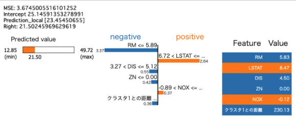
分析通り、RM、LSTATは重要度が高い数値を出している。
CHASは重要度が高いと見ていたが、低い数値となっている。単体では低い数値のため何かしらの変換が必要と思われる。

特徴量エンジニアリング

対応方針

• 正規分布への変換
  • MEDV： 予測残差の正規分布性を期待する分析アルゴリズム（線形回帰など）を使用するため、必要と考える。 また、目的変数にマイナス値が既に含まれてしまっているため、Box-Cox変換を用いる。 変換結果にマイナス値を含まれてしまい、線形モデルの評価時にエラーとなるため、Yeo-Johnson変換は行わない。　　
• 外れ値
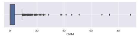
  • CRIM： （大きく外れた）外れ値（80）を含んでいる。犯罪率80%は疑わしい値。線形モデルを使用する（予定）のため、この外れ値を除去する。
• スケーリング
  • NOX, RM, DIS, PTRATIO, LSTAT, MEDV： （微妙な）外れ値の影響を軽減させたい 線形回帰に対しては有効でないと思われるが、非線形アルゴリズムをアンサンブルで使用する（予定）のため、有効であると考える。
• 特徴量生成
  • クラスタの重心からの距離： （まだ試してみたことがないため）実験的に効果検証してみる。

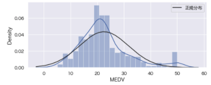
正規分布への変換

# 変換前の状態
import warnings
warnings.filterwarnings('ignore')
from scipy.stats import norm
plt.figure(figsize=[8,3])
sns.distplot(boston_df['MEDV'], kde=True, fit=norm, fit_kws={'label': '正規分布'}).grid()
plt.legend();

Yeo-Johnson変換

# Yeo-Johnson変換
from sklearn.preprocessing import PowerTransformer

yeo_johnson_df = boston_df.copy()
sk_yeojohnson = PowerTransformer(method='yeo-johnson') # インスタンス生成
yeojohnson_data = sk_yeojohnson.fit_transform(yeo_johnson_df[['MEDV']]) # 変換
yeo_johnson_df['MEDV'] = yeojohnson_data

import warnings
warnings.filterwarnings('ignore')
from scipy.stats import norm
plt.figure(figsize=[8,3])
sns.distplot(yeo_johnson_df['MEDV'], kde=True, fit=norm, fit_kws={'label': '正規分布'}).grid()
plt.legend()

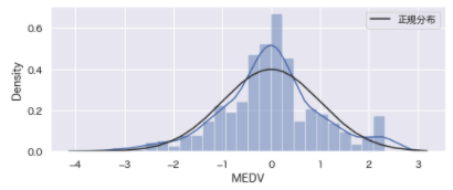
ランダムフォレストには効果があったが、線形モデルには適用できない。評価の過程で目的変数に負値を扱えないため。

Box-Cox変換

# Box-Cox変換 
from scipy.special import boxcox1p

boxcox_df = boston_df.copy()
lam=0.15
boxcox_df['MEDV'] = boxcox1p(boxcox_df['MEDV'], lam)

# 描画
plt.figure(figsize=[8,3])
sns.distplot(boxcox_df['MEDV'], kde=True, fit=norm, fit_kws={'label': '正規分布'}).grid()

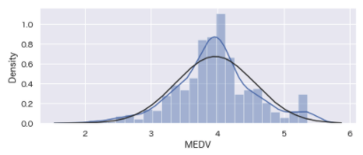
分布の偏りが軽減された。しかし非線形モデルには逆効果だった。

外れ値処理

# 確認
plt.figure(figsize=[10,2])
sns.boxplot(data=boston_df, x='CRIM').grid()

# 外れ値除去
boston_df.shape
boston_df = boston_df[boston_df['CRIM']<40]
boston_df = boston_df.reset_index()
boston_df.shape

# (506, 15)
# (500, 15)

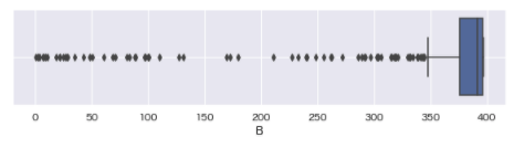
plt.figure(figsize=[10,2])
sns.boxplot(data=boston_df, x='B').grid()

# 外れ値除去
boston_df.shape
boston_df = boston_df[boston_df['B']>10]
boston_df = boston_df.reset_index()
boston_df.shape

# (500, 15)
# (493, 15)

スケーリング

col = ['NOX', 'RM', 'DIS', 'PTRATIO', 'LSTAT', 'MEDV']
boston_df[col].hist(bins=10, figsize=(10,8))

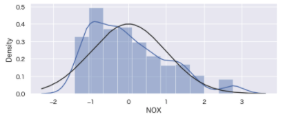
from sklearn.preprocessing import StandardScaler
# 標準化
scaler = StandardScaler()
boston_df['NOX'] = scaler.fit_transform(boston_df[['NOX']])

# 描画
plt.figure(figsize=[8,3])
sns.distplot(boston_df['NOX'], kde=True, fit=norm, fit_kws={'label': '正規分布'}).grid();

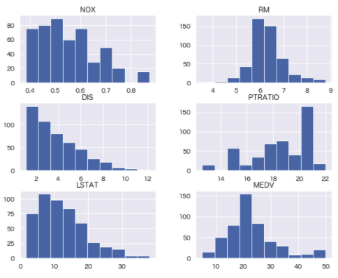
RM, DIS, PTRATIO, LSTAT, MEDVは、標準化しても精度に影響がなかったため、そのままとする。

特徴量生成

クラスタリング、主成分分析

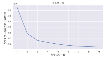
# クラスター数の探索（k-means++）
from sklearn.cluster import KMeans

def elbow(df):
    wcss = []
    for i in range(1, 10):
        kmeans = KMeans(n_clusters = i, init = 'k-means++', max_iter = 300, n_init = 30, random_state = 0)
        kmeans.fit(df.iloc[:, :])
        wcss.append(kmeans.inertia_)

    plt.figure(figsize=[8,4])
    plt.plot(range(1, 10), wcss)
    plt.title('エルボー法')
    plt.xlabel('クラスター数')
    plt.ylabel('クラスター内平方和（WCSS）')
    plt.grid()
    plt.show()

# 実行
elbow(boston_df)

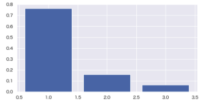
# 主成分分析
from sklearn.decomposition import PCA

# 寄与率
pca = PCA(n_components=3)
pca.fit(boston_df)
plt.figure(figsize=[8,4])
plt.grid()
plt.bar([n for n in range(1, len(pca.explained_variance_ratio_)+1)], pca.explained_variance_ratio_)

# 累積寄与率
contribution_ratio = pca.explained_variance_ratio_
accumulation_ratio = np.cumsum(contribution_ratio)
cc_ratio = np.hstack([0, accumulation_ratio])

plt.figure(figsize=[8,4])
plt.plot(accumulation_ratio, "-o")
plt.xlabel("主成分")
plt.ylabel("累積寄与率")
plt.grid()
plt.show()

contribution_ratios = pd.DataFrame(pca.explained_variance_ratio_)
contribution_ratios.round(decimals=2).astype('str').head()
print(f"累積寄与率：　{contribution_ratios[contribution_ratios.index<5].sum().round(decimals=2).astype('str').values}");

# 結果：累積寄与率：　['0.98']

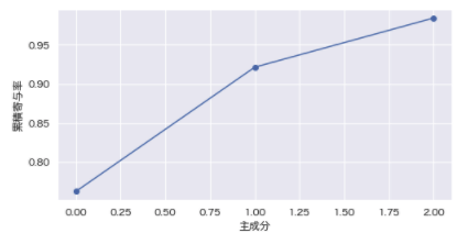
第３主成分までで寄与率は98%。クラスター数=3とする。

# クラスタリング（k-means）
from sklearn.preprocessing import StandardScaler

def clustering(df, num):
    sc = StandardScaler()
    sc.fit_transform(df)
    data_norm = sc.transform(df)

    cls = KMeans(n_clusters = num)
    result = cls.fit(data_norm)
    pred = cls.fit_predict(data_norm)

    plt.figure(figsize=[8, 4])
    sns.scatterplot(x=data_norm[:,0], y=data_norm[:,1], c=result.labels_)
    plt.scatter(result.cluster_centers_[:,0], result.cluster_centers_[:,1], s=250, marker='*', c='blue')
    plt.grid('darkgray')
    plt.show()

# 実行
clustering(boston_df, 3)

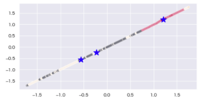
うまく分割できないため、主成分分析を行う。

## クラスタリング（k-means）＋主成分分析
from sklearn.decomposition import PCA

def cross(df, num):
    df_cls = df.copy()
    sc = StandardScaler()
    clustering_sc = sc.fit_transform(df_cls)

    # n_clusters：クラスター数
    kmeans = KMeans(n_clusters=num, random_state=42)
    clusters = kmeans.fit(clustering_sc)
    df_cls['cluster'] = clusters.labels_

    x = clustering_sc
    # n_components：削減結果の次元数
    pca = PCA(n_components=num)
    pca.fit(x)
    x_pca = pca.transform(x)
    pca_df = pd.DataFrame(x_pca)
    pca_df['cluster'] = df_cls['cluster']

    for i in df_cls['cluster'].unique():
       tmp = pca_df.loc[pca_df['cluster'] == i]
       plt.scatter(tmp[0], tmp[1])
    plt.grid()
    plt.show()

# 実行
cross(boston_df, 3)

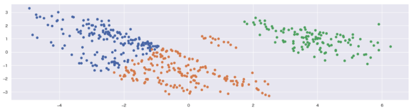
今度はうまく分割することができた。
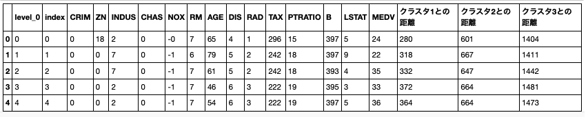
３つのクラスタと、その重心からの距離を算出する。

# 重心からの距離
def get_center_distance(df):
    num_cluster=3 # cluster数
    clusters = KMeans(n_clusters=num_cluster, random_state = 42)
    clusters.fit(df)
    centers = clusters.cluster_centers_

    columns = df.columns
    clust_features = pd.DataFrame(index = df.index)
    for i in range(len(centers)):
        clust_features['クラスタ' + str(i + 1) + 'との距離'] = (df[columns] - centers[i]).applymap(abs).apply(sum, axis = 1)
    return clust_features

# 実行
clust_features = get_center_distance(boston_df)
boston_df[clust_features.columns] = clust_features
boston_df.head()

オーバーサンプリング

# SMOTE
from imblearn.over_sampling import SMOTE

column = 'CHAS'
sm = SMOTE(random_state=42)
X = boston_df.drop(columns=column, axis=1)
y = boston_df[column]
X_sample, Y_sample = sm.fit_resample(X, y)

over_sampling = pd.DataFrame()
over_sampling = X_sample
over_sampling[column] = Y_sample

value_counts = over_sampling[column].value_counts()

df = pd.DataFrame()
df['ラベル'] = value_counts.index
df['件数'] = value_counts.values
ratio=[]
ratio.append((value_counts.values[0] / len(over_sampling[column]) * 100).round(decimals=2).astype('str'))
ratio.append((value_counts.values[1] / len(over_sampling[column]) * 100).round(decimals=2).astype('str'))
df['割合'] = [f'{ratio[0]}%', f'{ratio[1]}%']
print(f"全レコード数：{len(over_sampling[column])}")
df

# 全レコード数：916

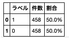
「CHAS」に対するオーバーサンプリングは、ランダムフォレストに対しては効果がある。その際「重心からの距離」がない方が精度が良い。
ただし、線形モデルに対しては、大幅な精度の悪化を招く。一旦、不採用とする。

カウント・エンコーディング

count_map = boston_df['CHAS'].value_counts().to_dict()
count_map

df = boston_df.copy()
df['CHASカウント'] = df['CHAS'].map(count_map)
df[['CHAS', 'CHASカウント']].head()
df = df.drop(columns='CHAS', axis=1)
sns.distplot(df['CHASカウント'])

# 結果：{0: 458, 1: 35}

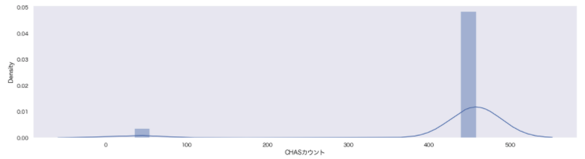
CAHSは住宅価格帯が異なるため、影響があると思ったが、得に影響はなかった。
出現頻度を学習させ、大小を明確にすれば影響が出ると考えたが、むしろ精度が悪化した。
一旦、このカウント・エンコーディングを採用するかは保留とする。

再評価

# 実行
rfr_model, y_test, y_pred = learning(RFR(random_state=42), boston_df)

決定係数（R2） = 0.924
平均絶対誤差（MAE） = 1.761
平均二乗誤差（MSE） = 5.588
対数平均二乗誤差（MSLE） = 0.018
平均二乗平方根誤差（RMSE） = 2.364
対数平方平均二乗誤差（RMSLE） = 0.134

# 線形回帰（重回帰）
from sklearn.linear_model import LinearRegression as LR
rfr_model, y_test, y_pred = learning(LR(), boston_df)

決定係数（R2） = 0.811
平均絶対誤差（MAE） = 2.919
平均二乗誤差（MSE） = 13.928
対数平均二乗誤差（MSLE） = 0.048
平均二乗平方根誤差（RMSE） = 3.732
対数平方平均二乗誤差（RMSLE） = 0.219

# 線形モデル
from sklearn.linear_model import Ridge
rfr_model, y_test, y_pred = learning(Ridge(), boston_df)

決定係数（R2） = 0.81
平均絶対誤差（MAE） = 2.924
平均二乗誤差（MSE） = 13.977
対数平均二乗誤差（MSLE） = 0.048
平均二乗平方根誤差（RMSE） = 3.739
対数平方平均二乗誤差（RMSLE） = 0.219

# 線形モデル
from sklearn.linear_model import Lasso
rfr_model, y_test, y_pred = learning(Lasso(), boston_df)

決定係数（R2） = 0.745
平均絶対誤差（MAE） = 3.172
平均二乗誤差（MSE） = 18.792
対数平均二乗誤差（MSLE） = 0.042
平均二乗平方根誤差（RMSE） = 4.335
対数平方平均二乗誤差（RMSLE） = 0.204

# 線形回帰（重回帰）
from sklearn.linear_model import ElasticNet
rfr_model, y_test, y_pred = learning(ElasticNet(), boston_df)

決定係数（R2） = 0.759
平均絶対誤差（MAE） = 3.112
平均二乗誤差（MSE） = 17.745
対数平均二乗誤差（MSLE） = 0.04
平均二乗平方根誤差（RMSE） = 4.212
対数平方平均二乗誤差（RMSLE） = 0.201

全体的に精度の向上が見られる。

特徴選択

# 実行
imp_df = rfr_importance(boston_df)
imp_df = imp_df.sort_values(by='重要度', ascending=False).reset_index().set_index("項目名")
imp_df = imp_df.drop(columns="index", axis=1)
imp_df

# 実行
boost_importance(boston_df)

# 実行
linear_importance(boston_df)

explain_importance(boston_df)

結果を踏まえて再評価

features = boston_df.drop(columns=['INDUS', 'CRIM', 'level_0', 'index', 'クラスタ3との距離']).columns

# 実行
rfr_model, y_test, y_pred = learning(RFR(random_state=42), boston_df[features])

決定係数（R2） = 0.929
平均絶対誤差（MAE） = 1.712
平均二乗誤差（MSE） = 5.248
対数平均二乗誤差（MSLE） = 0.017
平均二乗平方根誤差（RMSE） = 2.291
対数平方平均二乗誤差（RMSLE） = 0.129

# 線形回帰（重回帰）
from sklearn.linear_model import LinearRegression as LR
rfr_model, y_test, y_pred = learning(LR(), boston_df[features])

決定係数（R2） = 0.827
平均絶対誤差（MAE） = 2.803
平均二乗誤差（MSE） = 12.766
対数平均二乗誤差（MSLE） = 0.036
平均二乗平方根誤差（RMSE） = 3.573
対数平方平均二乗誤差（RMSLE） = 0.189

# 線形モデル
from sklearn.linear_model import Ridge
rfr_model, y_test, y_pred = learning(Ridge(), boston_df[features])

決定係数（R2） = 0.827
平均絶対誤差（MAE） = 2.799
平均二乗誤差（MSE） = 12.736
対数平均二乗誤差（MSLE） = 0.036
平均二乗平方根誤差（RMSE） = 3.569
対数平方平均二乗誤差（RMSLE） = 0.189

# 線形モデル
from sklearn.linear_model import Lasso
rfr_model, y_test, y_pred = learning(Lasso(), boston_df[features])

決定係数（R2） = 0.767
平均絶対誤差（MAE） = 3.124
平均二乗誤差（MSE） = 17.171
対数平均二乗誤差（MSLE） = 0.032
平均二乗平方根誤差（RMSE） = 4.144
対数平方平均二乗誤差（RMSLE） = 0.179

# 線形回帰（重回帰）
from sklearn.linear_model import ElasticNet
rfr_model, y_test, y_pred = learning(ElasticNet(), boston_df[features])

決定係数（R2） = 0.773
平均絶対誤差（MAE） = 3.073
平均二乗誤差（MSE） = 16.698
対数平均二乗誤差（MSLE） = 0.031
平均二乗平方根誤差（RMSE） = 4.086
対数平方平均二乗誤差（RMSLE） = 0.176

新宿の例といい、犯罪率は住宅価格との関係はないのかもしれない。
CHASは「０⇆１」で住宅価格が異なっていたため、影響はあると思われたが、「CHAS」単体では影響があまりなかった。

まとめ

実際に様々な手法を試して見て、効果があったもの、なかったものがあった。特に外れ値はどこまでを外れ値とするのかが判断が付けられず、モデル構築時の評価も加味して決めていきたい。
また過学習かどうかをまだ評価できていないため、モデル構築時（前）に確認することにします。

最後に

他の記事はこちらでまとめています。是非ご参照ください。

解析結果

実装結果：GitHub/boston_regression_preprocessing.ipynb
データセット：Boston House Prices-Advanced Regression Techniques

参考資料