Kraus表現を用いた量子ノイズを見ていき,それをQiskitを用いてシミュレートします.
Kraus表現
量子系の時間発展はTPCP写像で与えられますが,TPCP写像は
$$
\sum_{i=1}^m K_i^\dagger K_i =I
$$
を満たすKraus演算子$K_i$を用いて以下のように表せます.
$$
\rho\mapsto\sum_{i=1}^m K_i \rho K_i^\dagger
$$
このように時間発展を表現することをKraus表現と呼びます.
この後紹介する例の中では,初期状態を次のように定義します.
circ = QuantumCircuit(1)

circ.rx(np.pi / 3, 0)
circ.rz(np.pi / 4, 0)

state = DensityMatrix(circ)
plot_bloch_multivector(state)
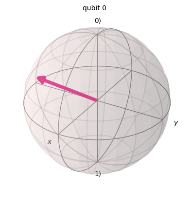
この状態に対し,いくつか代表的なノイズを作用させてみます.
Amplitude Damping Noise(自然放出)
Kraus演算子は
$$
\begin{align}
K_1&=|0\rangle\langle0|+\sqrt{1-p } |1\rangle\langle1| \\
K_2&=\sqrt{p}|0\rangle\langle1|
\end{align}
$$
です.
from qiskit.circuit import QuantumCircuit
from qiskit.quantum_info import DensityMatrix
from qiskit.visualization import plot_bloch_multivector

from qiskit.quantum_info import Kraus
from qiskit_aer.noise import amplitude_damping_error

p = 0.5

amp_error = Kraus(amplitude_damping_error(p))
print(amp_error)

#Kraus([[[-1.       +0.j,  0.       +0.j],
#        [ 0.       +0.j, -0.9539392+0.j]],
#
#       [[ 0.       +0.j,  0.3      +0.j],
#        [ 0.       +0.j,  0.       +0.j]]],
#      input_dims=(2,), output_dims=(2,))
確かに定義通りの演算子となっていることがわかります.実際に回路で作用させてみましょう.
circ = QuantumCircuit(1)

circ.rx(np.pi / 3, 0)
circ.rz(np.pi / 4, 0)
circ.append(amp_error, [0])

state = DensityMatrix(circ)
plot_bloch_multivector(state)
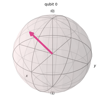
確かに,$|1\rangle$が$|0\rangle$に落ちていく様子が分かります.
Dephasing Noise(位相緩和)
Kraus演算子は
$$
\begin{aligned}
K_1&=\sqrt{1-\frac{p}{2}} I \\
K_2&=\sqrt{\frac{p}{2}} \sigma_z
\end{aligned}
$$
def dephasing_noise(p):
    return Kraus([np.array([[np.sqrt(1 - p / 2), 0],
        [0, np.sqrt(1 - p / 2)]], dtype = "complex128"),

       np.array([[np.sqrt(p / 2), 0],
        [0, -np.sqrt(p / 2)]], dtype = "complex128")])

circ = QuantumCircuit(1)

circ.rx(np.pi / 3, 0)
circ.rz(np.pi / 4, 0)
circ.append(dephasing_noise(p), [0])

state = DensityMatrix(circ)
plot_bloch_multivector(state)
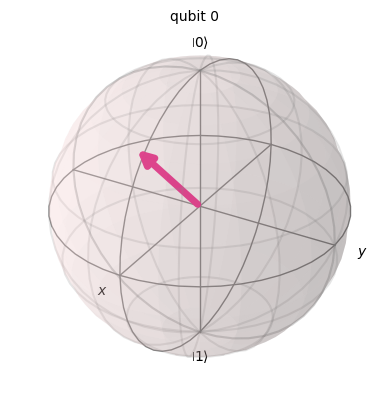
Z軸に近づいていっていることが分かります.
Depolarizing Noise(脱分極ノイズ)
Kraus演算子は
$$
K_1=\sqrt{1-\frac{3 \lambda}{4}} I,\ K_2=\sqrt{\frac{\lambda}{4}} X, \ K_3=\sqrt{\frac{\lambda}{4}} Y,\ K_4=\sqrt{\frac{\lambda}{4}} Z
$$
です.
def depolarizing_noise(p):
    return Kraus([np.array([[np.sqrt(1 - 3 * p / 4), 0],
        [0, np.sqrt(1 - 3 * p / 4)]], dtype = "complex128"),

       np.array([[np.sqrt(p / 4), 0],
        [0, -np.sqrt(p / 4)]], dtype = "complex128"),

       np.array([[0, np.sqrt(p / 4)],
        [np.sqrt(p / 4), 0]], dtype = "complex128"),

       np.array([[0, - 1j * np.sqrt(p / 4)],
        [1j * np.sqrt(p / 4), 0]], dtype = "complex128")])


circ = QuantumCircuit(1)

circ.rx(np.pi / 3, 0)
circ.rz(np.pi / 4, 0)
circ.append(depolarizing_noise(p), [0])

state = DensityMatrix(circ)
plot_bloch_multivector(state)
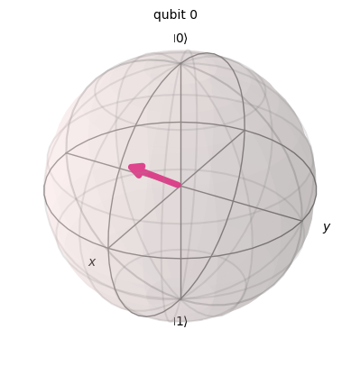
原点(=完全混合状態)に近づいていっていることがわかります.
ここで,depolarizing noiseはn個のqubitに対して
$$
\rho\mapsto(1-\lambda) \rho+\lambda \frac{I}{2^n}
$$
のように定義されることをコメントしておきます(Kraus表現はどうなるんでしょうか?).
コメント
dephasing, depolarizingでは自分でKraus演算子を定義しました.qiskit_aerを用いて
from qiskit_aer.noise import depolarizing_error, phase_damping_error
も実行できるのですが,dephasingのReferenceやdepolarizingのReferenceやには,上記とは異なるKraus演算子の定義がされています.
要するに,Kraus演算子は一意ではありません.ユニタリ行列$U$の成分を$U_{ij}$と表し,
$$
V_j := \sum_{i=1}^m U_{ji} K_i
$$
とすると,
$$
\begin{align}
\sum_{j=1}^m V_j \rho V_j^\dagger &=\sum_{j=1}^m \sum_{i=1}^m \sum_{k=1}^mU_{ji} K_i\rho U_{jk}^\ast K_k^\dagger \\
&=\sum_{i=1}^m K_i\rho K_i^\dagger
\end{align}
$$
となり,確かに写像先が同じになっていることが分かります.また完全性も同様に満たしていることが分かります.
最後に
今回はKraus表現を用いてノイズを自作してみました.
Version Information
| Software | Version |
|---|---|
| qiskit | 0.45.0 |
| System information | |
|---|---|
| Python version | 3.10.12 |