試験の数理 その4(問題paramter推定の実装) の続きです。
前回は、「3PL modelの問題paramter推定の実装について」でした。
今回は、「受験者の能力parameter の推定」です。
用いた環境は、
- python 3.8
- numpy 1.19.2
- matplotlib 3.3.1
です。
理論
問題設定
問題パラメータ$a, b, c$が既知であるときに、問題に対する反応ベクトル$u_j$から3PL modelの受験者parameter $\theta_j$を推定することとなります。
目的関数
ここでは、最尤推定で解くこととします。$P_{ij}$を3PL modelで問題$i$に受験者$j$が正答する確率、$Q_{ij} = 1 - P_{ij}$としたときに尤度は
\begin{align}
\Pr\{U_j = u_j|\theta_j, a, b, c\} &= \prod_{i} \Pr\{U_{ij} = u_{ij}|\theta, a, b, c\}\\
&= \prod_{i}P_{ij}^{u_{ij}}Q_{ij}^{1-u_{ij}}
\end{align}
となるので、対数尤度は
\begin{align}
\mathcal{L}(u_j, \theta_j, a, b, c) &= \ln \Pr\{U_j = u_j|\theta_j, a, b, c\}\\
&= \sum_{i}u_{ij}\ln P_{ij} + (1-u_{ij})\ln Q_{ij}
\end{align}
となります。ここで、目的のparamter $\hat{\theta_j}$は
\begin{align}
\hat{\theta_j} = \arg \max_{\theta}\mathcal{L}(u_j, \theta, a, b, c)
\end{align}
となります。
微分係数
問題を解くために微係数を計算しておきます。$\partial_\theta := \frac{\partial}{\partial \theta}$としたとき、
\begin{align}
\partial_\theta\mathcal{L}(u_j, \theta, a, b, c) &= \sum_i a_i\left(\frac{u_{ij}}{P_{ij}} - 1\right)P_{ij}^* \\
\partial_\theta^2\mathcal{L}(u_j, \theta, a, b, c) &= \sum_i a_i^2\left(\frac{c_iu_{ij}}{P_{ij}^2} - 1\right)P_{ij}^* Q_{ij}^*
\end{align}
となります。ここで$P^*_{ij}, Q^*_{ij}$は2PL modelで問題$i$に受験者$j$が正答する確率です。ここから、解では、$\partial_\theta\mathcal{L} = 0, \partial_\theta^2\mathcal{L} < 0$となっているはずです。
解法
ここでは、Newton Raphson法を用いて、計算を行います。具体的な手順は以下のとおりです。
- $\theta$として乱数で値を決める。
- $\theta^{(new)} = \theta^{(old)} - \partial_\theta\mathcal{L}(\theta^{(old)})/\partial_\theta^2\mathcal{L}(\theta^{(old)})$で値を逐次更新し、$\partial_\theta\mathcal{L} < \delta$の時、終了する。
- $\partial_\theta^2\mathcal{L} < 0$となっているか、および値が発散していないか判定し、条件に満たない場合1からやりなおす。
- $N$回やりなおしても値が見つからない場合、解なしとする。
実装
pythonを用いて次のように実装しました。
import numpy as np
from functools import partial

# 定数の定義 delta: 収束判定、 Theta_: 発散判定、 N:繰り返し判定
delta = 0.0001
Theta_ = 20
N = 20
def search_theta(u_i, item_params, trial=0):
    # 繰り返しが規定回数に到達したらNoneを返す
    if trial == N:
        return None
    # thetaを乱数で決める。
    theta = np.random.uniform(-2, 2)
    # NR法
    for _ in range(100):
        P3_i = np.array([partial(L3P, x=theta)(*ip) for ip in item_params])
        P2_i = np.array([partial(L2P, x=theta)(*ip) for ip in item_params])
        a_i = item_params[:, 0]
        c_i = item_params[:, 2]
        res = (a_i *( u_i / P3_i - 1) * P2_i).sum()
        d_res = (a_i * a_i * ( u_i  * c_i/ P3_i / P3_i  - 1) * P2_i * (1 - P2_i)).sum()
        theta -= res/d_res
        # 収束判定
        if abs(res) < delta:
            if d_res < -delta and -Theta_ < theta < Theta_:
                return theta
            else:
                break
    return search_theta(u_i, item_params, trial + 1)
実行と結果
上の関数を用いて数値計算を行いました。実行には問題parameterとして前回の推定結果の
| a / 識別力 | b / 困難度 | c / 当て推量 | |
|---|---|---|---|
| 問 1 | 3.49633348 | 1.12766137 | 0.35744497 |
| 問 2 | 2.06354365 | 1.03621881 | 0.20507606 |
| 問 3 | 1.64406087 | -0.39145998 | 0.48094315 |
| 問 4 | 1.47999466 | 0.95923840 | 0.18384673 |
| 問 5 | 1.44474336 | 1.12406269 | 0.31475672 |
| 問 6 | 3.91285332 | -1.09218709 | 0.18379076 |
| 問 7 | 1.44498535 | 1.50705016 | 0.20601461 |
| 問 8 | 2.37497907 | 1.61937999 | 0.10503096 |
| 問 9 | 3.10840278 | 1.69962392 | 0.22051818 |
| 問 10 | 1.79969976 | 0.06053145 | 0.29944448 |
を用いました。
params = np.array(
    [[ 3.49633348,  1.12766137,  0.35744497],
     [ 2.06354365,  1.03621881,  0.20507606],
     [ 1.64406087, -0.39145998,  0.48094315],
     [ 1.47999466,  0.9592384 ,  0.18384673],
     [ 1.44474336,  1.12406269,  0.31475672],
     [ 3.91285332, -1.09218709,  0.18379076],
     [ 1.44498535,  1.50705016,  0.20601461],
     [ 2.37497907,  1.61937999,  0.10503096],
     [ 3.10840278,  1.69962392,  0.22051818],
     [ 1.79969976,  0.06053145,  0.29944448]]
)
さて、受験者paramterの推定についてですが、実は今回は問題数が10しかなく、入力としてありえる受験結果は[0, 0, ..., 0]から[1, 1, ..., 1] の1024通りしかありません。実際問題の応答は正誤の2通りしかないのですから、ありえる入力は問題数を$I$とすれば、$2^I$ 通りになってしまいます。それゆえ、実数parameter$\theta$を完全に精度良くみることは不可能です。例えば、ある受験者のparameterが0.1224程度だっとし、そこから、[0, 1, 1, 0, 1, 1, 1, 0, 0, 1]という結果を得たとしましょう。ここで、
search_theta(np.array([0, 1, 1, 0, 1, 1, 1, 0, 0, 1]), params)
と計算すると、結果は0.8167程度となります。グラフにplotすると次のようになります。
import matplotlib.pyplot as plt
y = []
y_ = []
x = np.linspace(-3, 3, 201)
u_ = np.array([0, 1, 1, 0, 1, 1, 1, 0, 0, 1])
for t in x:
    theta = t
    P3_i = np.array([partial(L3P, x=theta)(*ip) for ip in params])
    P2_i = np.array([partial(L2P, x=theta)(*ip) for ip in params])
    a_i = params[:, 0]
    # 対数尤度
    res = (u_ * np.log(P3_i) + (1 - u_) * np.log(1 - P3_i)).sum()
    # 微分係数
    res_ = (a_i *( u_ / P3_i - 1) * P2_i).sum()
    y.append(res)
    y_.append(res_)


# plot
# 微分係数
plt.plot(x, y_, label="dL")
plt.plot(x, x * 0, label="0")
plt.xlabel("theta")
plt.ylabel("val")
plt.legend()
plt.show()
# 対数尤度
plt.plot(x, y, label="L")
plt.xlabel("theta")
plt.ylabel("val")
plt.legend()
plt.show()
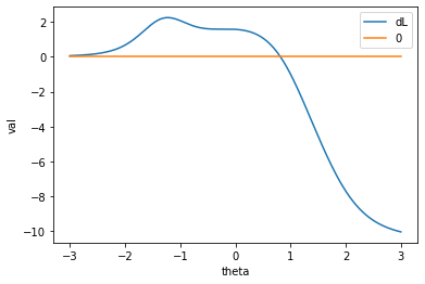
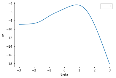
実際は0.1224程度だったので、かなり高い数値となります。これは、問2や問5などを運良く正解できたことによります。これは問題数が少なかったことによると思われるので、問題数がより多ければ、より精度の良い推定が得られやすくなるでしょう。
おまけ
入力にもちいるbinaryですが、たとえば、
n_digits = 10
num = 106
u_ = np.array([int(i) for i in f'{num:0{n_digits}b}'])
とすれば、array([0, 0, 0, 1, 1, 0, 1, 0, 1, 0])などと得ることができます。0 <= num <= 1023
全入力に対する最適値をこれでみることができます。ただし、[1, 1, ..., 1]などいくつかはまともな値を得られません。
結び
5記事に渡って書いた「試験の数理」シリーズですが、今回で一応の完結です。この記事やこれまでの記事をを見てくださり、ありがとうございました。
項目反応理論は奥が深く、例えば、全部に答えてくれていない(歯抜けの)データはどうするんだ?とかそもそもバイナリでなくて多段階だったり、実数値でデータが出ている場合にはどうなんだ?とか様々な応用や発展が考えられます。また機会があればそのあたりも勉強して記事にしたいと思っています。
なにか、質問やつっこみなどがありましたら、気軽にコメントなり修正依頼などを出していただければ嬉しいです。