PyroでDeep Kernel Learning

Deep Kernel Learningは深層学習とガウス過程の組み合わせた手法で、ベイズ深層学習の１つになります。
方法としては、ガウス過程のカーネルの入力にディープニューラルネット(DNN)から出力された特徴量を用いてdeep kernelを作成しています。
数式としては以下のような感じです。

k_{deep}(x,x') = k(f(x),f(x'))

ガウス過程が無限ユニットを持つニューラルネットと等価なので、イメージ的にはDNNの最後にもう一層追加されたような感じです。
以前の記事で試したように、ガウス過程ではカーネルのハイパーパラメータを最適化させることが重要です。
Deep Kernel Learningでは、DNNのパラメータとカーネルのハイパーパラメータを同時に最適化して学習するようです。

詳細は下記の論文を参照してください。
[1] Deep Kernel Learning, 2015, Andrew G. Wilson et al.,https://arxiv.org/abs/1511.02222
[2] Stochastic Variational Deep Kernel Learning, 2016, Andrew G. Wilson et al., https://arxiv.org/abs/1611.00336

参考文献
Bingham, E., Chen, J. P., Jankowiak, M., Obermeyer, F., Pradhan, N., Karaletsos, T. et al. (2019).
Pyro: Deep universal probabilistic programming. The Journal of Machine Learning Research, 20(1), 973-978.
コードは以下にあるものを改変して使用しています。
https://github.com/pyro-ppl/pyro (Apache-2.0 License)

Deep Kernel LearningでMNISTを学習してみる

Pyroでは、gp.kernels.Warpingクラスを使うことで簡単にdeep kernelを作成できます。
Pyroの公式チュートリアルにDeep Kernel Learningのコードがあったので、それを参考に学習してみます。

import numpy as np
import torch
import torch.nn as nn
import torch.nn.functional as F
import torchvision
from torchvision import transforms
import pyro
import pyro.contrib.gp as gp
import pyro.infer as infer

MNISTはデータ数が多いので、ミニバッチで学習します。
データセットを設定します。

batch_size = 100
transform = transforms.Compose([transforms.ToTensor(),transforms.Normalize((0.5, ), (0.5, ))])
trainset = torchvision.datasets.MNIST(root='./data', train=True, download=True, transform=transform)
trainloader = torch.utils.data.DataLoader(trainset, batch_size=batch_size, shuffle=True)
testset = torchvision.datasets.MNIST(root='./data', train=False, download=True, transform=transform)
testloader = torch.utils.data.DataLoader(testset, batch_size=batch_size, shuffle=False)

まずは、通常のDNNのモデルを用意します。

class CNN(nn.Module):
    def __init__(self):
        super().__init__()
        self.conv1 = nn.Conv2d(1, 10, kernel_size=5)
        self.conv2 = nn.Conv2d(10, 20, kernel_size=5)
        self.fc1 = nn.Linear(320, 50)
        self.fc2 = nn.Linear(50, 10)
    def forward(self, x):
        x = F.relu(F.max_pool2d(self.conv1(x), 2))
        x = F.relu(F.max_pool2d(self.conv2(x), 2))
        x = x.view(-1, 320)
        x = F.relu(self.fc1(x))
        x = self.fc2(x)
        return x

これにカーネルをラップしてdeep kernelを作成します。

rbf = gp.kernels.RBF(input_dim=10, lengthscale=torch.ones(10))
deep_kernel = gp.kernels.Warping(rbf, iwarping_fn=CNN())

ガウス過程の計算コストを少なくするためスパース近似を用います。
スパース近似では誘導点(inducing point)を用いますが、今回はバッチサイズ1つ分のトレーニングデータにします。

Xu, _ = next(iter(trainloader))
likelihood = gp.likelihoods.MultiClass(num_classes=10)
gpmodule = gp.models.VariationalSparseGP(X=None, y=None, kernel=deep_kernel, Xu=Xu, likelihood=likelihood, latent_shape=torch.Size([10]), num_data=60000)
optimizer = torch.optim.Adam(gpmodule.parameters(), lr=0.01)
elbo = infer.TraceMeanField_ELBO()
loss_fn = elbo.differentiable_loss

ミニバッチ学習の関数を定義します。

def train(train_loader, gpmodule, optimizer, loss_fn, epoch):
    total_loss = 0
    for data, target in train_loader:
        gpmodule.set_data(data, target)
        optimizer.zero_grad()
        loss = loss_fn(gpmodule.model, gpmodule.guide)
        loss.backward()
        optimizer.step()
        total_loss += loss
    return total_loss / len(train_loader)

def test(test_loader, gpmodule):
    correct = 0
    for data, target in test_loader:
        f_loc, f_var = gpmodule(data)
        pred = gpmodule.likelihood(f_loc, f_var)
        correct += pred.eq(target).long().sum().item()
    return 100. * correct / len(test_loader.dataset)

学習を行います。

import time
losses = []
accuracy = []
epochs = 10
for epoch in range(epochs):
    start_time = time.time()
    loss = train(trainloader, gpmodule, optimizer, loss_fn, epoch)
    losses.append(loss)
    with torch.no_grad():
        acc = test(testloader, gpmodule)
    accuracy.append(acc)
    print("Amount of time spent for epoch {}: {}s\n".format(epoch+1, int(time.time() - start_time)))
print("loss:{:.2f}, accuracy:{}".format(losses[-1],accuracy[-1]))

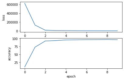
1エポックを約30秒で学習できました。
最終的なaccuracyは96.23%でした。(公式チュートリアルでは99.41%にまで出来るようです。)
学習曲線を表示します。

import matplotlib.pyplot as plt
plt.subplot(2,1,1)
plt.plot(losses)
plt.xlabel("epoch")
plt.ylabel("loss")
plt.subplot(2,1,2)
plt.plot(accuracy)
plt.xlabel("epoch")
plt.ylabel("accuracy")

テスト画像と予測出力を並べて見てみます。

data, target = next(iter(testloader))
f_loc, f_var = gpmodule(data)
pred = gpmodule.likelihood(f_loc, f_var)
for i in range(len(data)):
    plt.subplot(1,2,1)
    plt.imshow(data[i].reshape(28, 28))
    plt.subplot(1,2,2)
    plt.bar(range(10), f_loc[:,i].detach(), yerr= f_var[:,i].detach())
    ax = plt.gca()
    ax.set_xticks(range(10))
    plt.xlabel("class")
    plt.savefig('image/figure'+ str(i) +'.png')
    plt.clf()

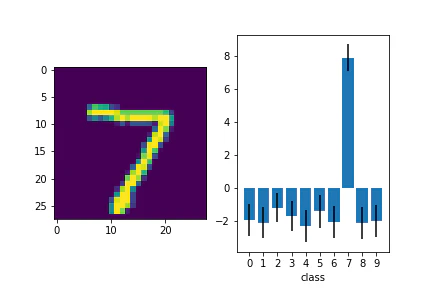
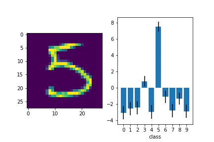
青い棒が平均値で、エラーバーが分散を表しています。
10クラスそれぞれに出力があり、正解のクラスで高い値が出力されていることがわかりました。

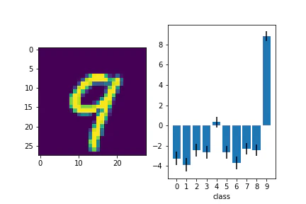
判別が難しい画像についても見てみます。



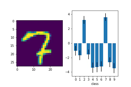
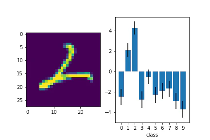
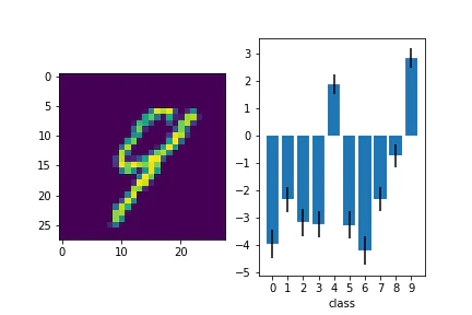
複数のクラスで出力が高いですね。エラーバーも考えると有意に差がないようにも見えます。

終わりに

通常のDeep Learnigのように学習することができました。
出力として平均値と分散を出すことが出来るのが、通常のDeep Learnigには無い利点だと思います。
似たものとしてガウス過程を積み重ねた深層ガウス過程(DGP)もあるので、そちらも勉強したいですね。