Finding a shortest path using a specific street network is a common GIS problem that has many practical applications. For example, navigation, one of those ‘every-day’ applications for which routing algorithms are used to find the optimal route between two or more points.
Of course, the Python ecosystem has produced packages that can be used to conduct network analyses, such as routing. The NetworkX package provides various tools to analyse networks, and implements several different routing algorithms, such as the Dijkstra’s or the A* algorithms. Both are commonly used to find shortest paths along transport networks.
To be able to conduct network analysis, it is, of course, necessary to have a network that is used for the analyses. The OSMnx package enables us to retrieve routable networks from OpenStreetMap for various transport modes (walking, cycling and driving). OSMnx also wraps some of NetworkX’s functionality in a convenient way for using it on OpenStreetMap data.
In the following section, we will use OSMnx to find the shortest path between two points based on cyclable roads. With only the tiniest modifications, we can then repeat the analysis for the walkable street network.
特定のストリートネットワークの最短経路を探すことは、実践的な要素を持つ、一般的なGISの課題です。例えば、ナビゲーションは、2点以上の間の最適経路を求めるためにルーティングアルゴリズムが使われる日常的アプリケーションのひとつである。
もちろん、Pythonのエコシステムは、ネットワーク分析に使われるパッケージを作成している、例えば、ルーティングのような。 NetworkXパッケージは、ネットワーク分析用の様々なツール提供し、いくつかの異なるルーティングのアルゴリズムを実装している、例えば、ダイクストラ法 や、A*(エースター)探索アルゴリズムなど。いずれも、交通網の最短経路を探すために、一般的に使われます。
ネットワーク分析を実施するには、もちろん、分析するネットワークが必要です。OSMnxパッケージによって、私たちは、オープンストリートマップから、様々な交通のモード(徒歩、自転車、車)で、ルーティング可能なネットワークを取得できます。また、OSMnxは、いくつかのNetworkXの機能を、オープンストリートマップ上で使用しやすいように、ラップします。
このセクションでは、自転車で走行できる道路の2つの座標の最短経路を見つけるために、OSMnxを使います。そこからのちょっとした修正で、私たちは徒歩移動可能なストリートネットワークの分析も行うことができます。
Obtain a routable network
To download OpenStreetMap data that represents the street network, we can use it’s
graph_from_place() <https://osmnx.readthedocs.io/en/stable/osmnx.html#osmnx.graph.graph_from_place>__ function. As parameters, it expects a place name and, optionally, a network type.
ストリートネットワークを表現するオープンストリートマップをダウンロードするために、私たちはgraph_from_place()関数を使うことができます。この関数のパラメータは、場所の名前と、(オプションで)ネットワークタイプです。
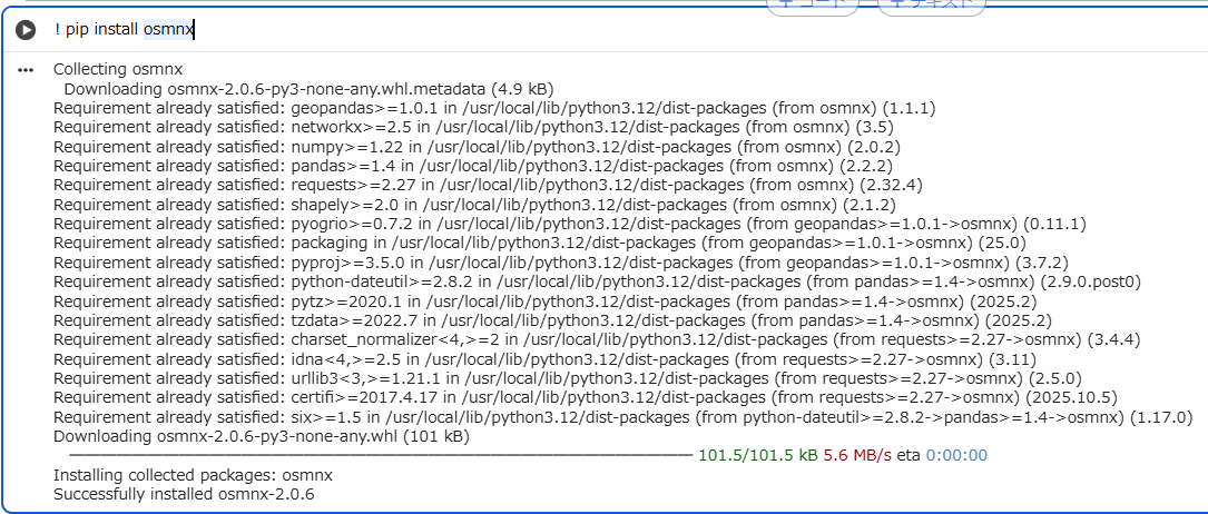
では実践です。まず、osmnxをインストールします。
! pip install osmnx
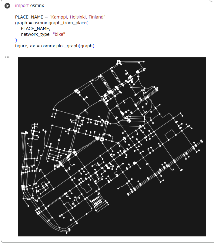
graph_from_place()でストリートネットワークを取得し、それをplot_graph関数でプロットします。
import osmnx

PLACE_NAME = "Kamppi, Helsinki, Finland"
graph = osmnx.graph_from_place(
    PLACE_NAME,
    network_type="bike"
)
figure, ax = osmnx.plot_graph(graph)
Pro tip!
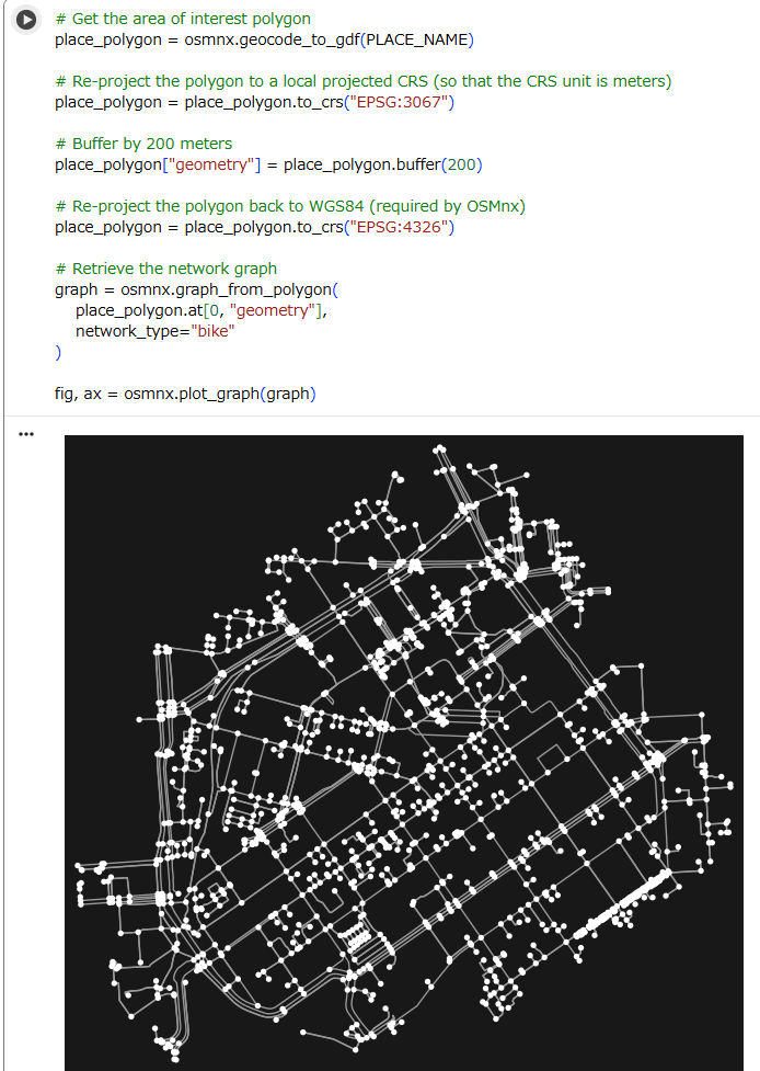
Sometimes the shortest path might go slightly outside the defined area of interest. To account for this, we can fetch the network for a bit larger area than the district of Kamppi, in case the shortest path is not completely inside its boundaries.
時々、最短経路は、興味があるエリアのわずかに外側になることがあります。
これを考慮し、最短経路がエリアの境界線の内側に収まらないケースを想定し、私たちは、Kamppi地区より少しだけ大きなエリアのネットワークを取得できす。
# Get the area of interest polygon
place_polygon = osmnx.geocode_to_gdf(PLACE_NAME)

# Re-project the polygon to a local projected CRS (so that the CRS unit is meters)
place_polygon = place_polygon.to_crs("EPSG:3067")

# Buffer by 200 meters
place_polygon["geometry"] = place_polygon.buffer(200)

# Re-project the polygon back to WGS84 (required by OSMnx)
place_polygon = place_polygon.to_crs("EPSG:4326")

# Retrieve the network graph
graph = osmnx.graph_from_polygon(
    place_polygon.at[0, "geometry"],
    network_type="bike"
)

fig, ax = osmnx.plot_graph(graph)
Data overview
Now that we obtained a complete network graph for the travel mode we specified (cycling), we can take a closer look at which attributes are assigned to the nodes and edges of the network. It is probably easiest to first convert the network into a geo-data frame on which we can then use the tools we learnt in earlier lessons.
To convert a graph into a geo-data frame, we can use osmnx.graph_to_gdfs() (see previous section). Here, we can make use of the function’s parameters nodes and edges to select whether we want only nodes, only edges, or both (the default):
さて、私たちは、指定した交通のモード(自転車)についての完全なネットワークグラフを取得したので、ネットワークのノードとエッジにどの属性が割り当てられたか、をより細かく見ることができます。
それは、おそらく、以前のレッスンで学んだツールを使ってネットワークをGeoDataFrameにコンバートするよりも、はるかに簡単です。
グラフをGeoDataFrameに変換するため、osmnx.graph_to_gdfs()関数を使います。(以前のレッスンを参照ください。)
ここでは、ノードだけ、エッジだけ、もしくはその両方(デフォルト)を選択するために、関数のパラメータのnodesとedgesを使います。
# Retrieve only edges from the graph
edges = osmnx.graph_to_gdfs(graph, nodes=False, edges=True)
edges.head()
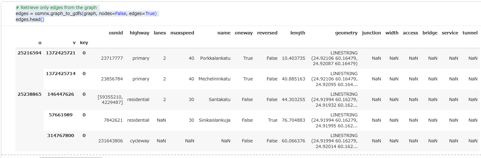
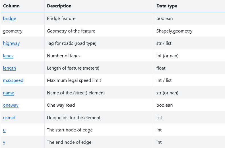
The resulting geo-data frame comprises of a long list of columns. Most of them relate to OpenStreetMap tags, and their names are rather self-explanatory. the columns u and v describe the topological relationship within the network: they denote the start and end node of each edge.
結果のGeoDataFrameは、多くの列により構成されます。列の多くはオープンストリートマップのタグに紐づき、それらの名前は、むしろ、説明不要です。uとvで、ネットワーク内のトポロジーの関連(それぞれのエッジの開始と終了のノード)を表現します。
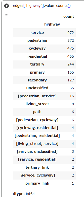
What types of streets does our network comprise of?
私たちのネットワークは、どのストリートのタイプにより構成されているでしょうか?
edges["highway"].value_counts()
Transform to projected reference system
The network data’s cartographic reference system (CRS) is WGS84 (EPSG:4326), a geographic reference system. That means, distances are recorded and expressed in degrees, areas in square-degrees. This is not convenient for network analyses, such as finding a shortest path.
Again, OSMnx’s graph objects do not offer a method to transform their geodata, but OSMnx comes with a separate function:
osmnx.project_graph() <https://osmnx.readthedocs.io/en/stable/osmnx.html#osmnx.projection.project_graph>__ accepts an input graph and a CRS as parameters, and returns a new, transformed, graph. If crs is omitted, the transformation defaults to the locally most appropriate UTM zone.
ネットワークデータのCRSは、測地系の一つである、WGS84(EPSG:4326)です。
つまり、距離は度で、面積は平方度で、記録・表現されます。
これは、最短経路の検出などのネットワーク分析にとって都合が悪いです。
今一度、OSMnxのグラフのオブジェクトはその地理空間データを変換する方法を提供しません。しかし、OSMnxには、osmnx.project_graph()関数があります。この関数は、グラフとCRSを入力パラメータとして、新しく変換されたグラフを返します。パラメータcrsが省略された場合、デフォルトでその地域の最も適切なUTMゾーンに変換します。
# Transform the graph to UTM
graph = osmnx.project_graph(graph)

# Extract reprojected nodes and edges
nodes, edges = osmnx.graph_to_gdfs(graph)

nodes.crs
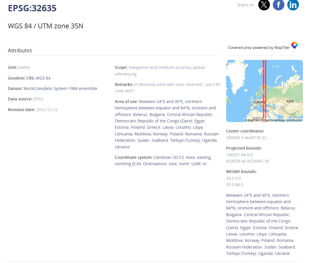
結果はこうなりました。
<Projected CRS: EPSG:32635>
Name: WGS 84 / UTM zone 35N
Axis Info [cartesian]:
- E[east]: Easting (metre)
- N[north]: Northing (metre)
Area of Use:
- name: Between 24°E and 30°E, northern hemisphere between equator and 84°N, onshore and offshore. Belarus. Bulgaria. Central African Republic. Democratic Republic of the Congo (Zaire). Egypt. Estonia. Finland. Greece. Latvia. Lesotho. Libya. Lithuania. Moldova. Norway. Poland. Romania. Russian Federation. Sudan. Svalbard. Türkiye (Turkey). Uganda. Ukraine.
- bounds: (24.0, 0.0, 30.0, 84.0)
Coordinate Operation:
- name: UTM zone 35N
- method: Transverse Mercator
Datum: World Geodetic System 1984 ensemble
- Ellipsoid: WGS 84
- Prime Meridian: Greenwich
UTMゾーン35Nという結果は妥当に見えます。
Analysing network properties
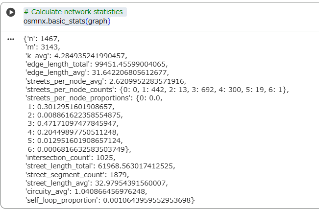
Now that we have prepared a routable network graph, we can turn to the more analytical features of OSMnx, and extract information about the network. To compute basic network characteristics, use
osmnx.basic_stats() <https://osmnx.readthedocs.io/en/stable/osmnx.html#osmnx.stats.basic_stats>__:
ネットワークのルートテーブルを用意しましたので、OSMnxのより分析的な機能に目を向け、ネットワークについての情報を抽出することができます。基本的なネットワークの特性を計算するために、osmnx.basic_stats()関数を使います。
# Calculate network statistics
osmnx.basic_stats(graph)
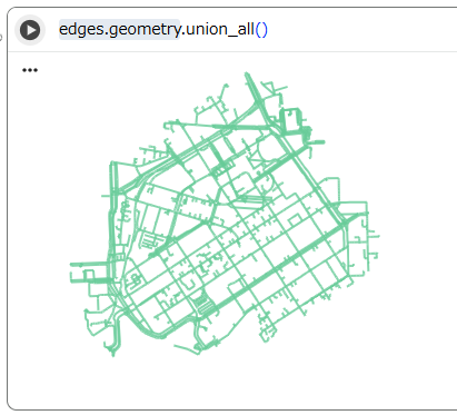
This does not yet yield all interesting characteristics of our network, as OSMnx does not automatically take the area covered by the network into consideration. We can do that manually, by, first, delineating the complex hull of the network (of an ’unary’ union of all its features), and then, second, computing the area of this hull.
OSMnxは自動ではネットワークによりカバーされたエリアを考慮しないので、私たちのネットワークについて、まだすべての興味深い特性を出力していません。
私たちはそれを手動で行うことができます。
まず、最初にネットワークの(「単一」の特徴の)凸包の輪郭を描きます。次に、その外側のエリアを計算します。
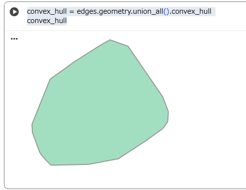
convex_hull = edges.geometry.union_all().convex_hull
convex_hull
妥当性が不明なので、union_all()だけしてみましょう。
良さそうです。では、凸包の統計情報を見てみましょう。
stats = osmnx.basic_stats(graph, area=convex_hull.area)
stats
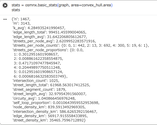
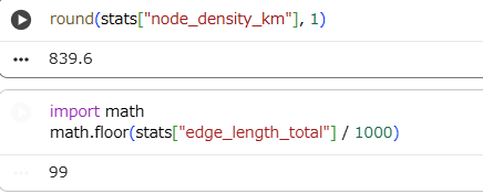
As we can see, now we have a lot of information about our street network that can be used to understand its structure. We can for example see that the average node density in our network is {glue:}node_density_km nodes/km and that the total edge length of our network is more than {glue:}edge_length_total kilometers.
ご覧の通り、その構造を理解するために使われる、たくさんのストリートネットワークの情報が取得できています。
例えば、ネットワークの平均的なノードの密度('node_density_km')は約839.6 km、ネットワークのエッジのトータルの長さ('edge_length_total)は約99 kmであることがわかります。
Note: Centrality measures
In earlier years, this course also discussed degree centrality. Computing network centrality has changed in OSMnx: going in-depth would be beyond the scope of this course. Please see the OSMnx notebook for an example.
中心性の測定
昔は、このコースは中心性の度合いについても議論しました。OSMnxにおけるネットワークの中心性を計算は変わりました。詳しく調べることは、このコースの範囲を超えかねません。 例として、OSMnx notebookを見てください。