Kernel t-SNEを使ったデータの分類をフルスクラッチ実装でやってみた

$ $
本記事で取り扱う内容は下記の3点となります．

• SNE の理論と実装
• $t$-SNE の理論と実装
• Kernel $t$-SNE の理論と実装

$ $本記事では Kernel $t$-SNE によりデータを分類することを目標としますが，その過程において，SNE，$t$-SNE の理論と Python による実装例もご紹介したいと思います．

はじめに

機械学習手法の一つであるクラスタリング (Clustering) や分類 (Classification) は実社会の様々な場面で活用されています．
例えば次のような活用例が挙げられ，実は私達の身近なところで使われていることがわかります．

• 顧客タイプを分類しマーケティングやセールスへ活用
• スパムメールのフィルタリング
• 株価予測
• 悪意のある金融取引の検知

なお，クラスタリング (Clustering) と分類 (Classification) は異なり

• ラベル付されていないデータを用いた教師なし学習が Clustering
• ラベル付されたデータを用いた教師あり学習が Classification

$ $となります．
この違いは $t$-SNE と Kernel $t$-SNE の違いにもなるのでぜひ理解していただきたいです．

さて，実社会においてこのような適用例がありますと言うのは簡単ですが．これらを自分でやりたい！となった時みなさんはどうしますか？
恐らく Scikit-learn，TensorFlow，Chainer，PyTorch，などなどライブラリやモジュールを使用することが多いのではないでしょうか．
私の場合は以下のような事情があったためフルスクラッチで実装しました．同じような状況にある方も多いのではないかと思います．

1. 諸事情からモジュールを使えない
2. 既存のモジュールとは異なるアルゴリズムを使いたい
3. 計算の途中経過の出力など，プログラムを頻繁に修正する予定がある

本記事では，数あるクラスタリング手法の中から SNE (Stochastic Neighbor Embedding) と呼ばれる手法を取り上げます．
はじめに SNE とは何かについて簡単な説明を行い，その後で計算方法と Python による実装例をご紹介します．

1. SNEとは

$ $SNE (Stochastic Neighbor Embedding) は HintonとRoweisにより提案されたクラスタリング手法です．
SNE では高次元空間におけるデータの近傍性 (neighborhood identity) を最大限保ったまま低次元空間へと埋め込む，すなわち次元削減することを目標としています．
３次元空間に生きる人間にとって４次元以上のデータ同士の類似度を知ることは容易ではありませんが，次元削減により２次元や３次元空間へ埋め込んでしまえば容易に可視化することができます．

$ $$t$-SNE (t-distributed Stochastic Neighbor Embedding) は SNE の改良版として Maaten と Hinton により提案された手法です．
低次元空間におけるデータの類似度を計算する際に，SNEではガウス関数を使用しますが $t$-SNE ではスチューデントの $t$ 分布を使用します．

$ $SNE や $t$-SNE では全てのデータセットを用いてクラスタリングを行うため，新たなデータが加わったときに再度全データを用いて計算を回さなければなりません．
データ数と次元が小さければそれでも良いかもれませんが，データ数や次元が大きくなると計算時間も増えるためこれでは実用に耐えれません．
Kernel $t$-SNE では新規データが加わった際に学習済みのクラスタリング結果を用いて新規データの分類を行うことができるため，計算時間が増加するということはありません．この点が Kernel $t$-SNE の特徴になります．
Kernel $t$-SNE は Out-of-Sample Kernel Extensions for Nonparametric Dimensionality Reduction において，Gisbrechtらによって提案されました．

2. 理論

$ $ここでは SNE, $t$-SNE, Kernel $t$-SNE の理論について説明します．
本記事ではプログラムの実装に重点を置いているため，理論的な解説は省略し簡単に計算方法のみ示します．
理論的，数学的な理解を深めたい方は例えば下記のようなサイトや参考文献をご参照ください．

• 高次元のデータを可視化するt-SNEの効果的な使い方
• t-SNE clearly explained
• t-SNEを理解して可視化力を高める

2.1 SNE の理論

$ $ここでは SNE の計算方法について解説します．
SNE における最終的な目標は下記のように高次元空間に属するデータ行列 $X$ の次元を削減することです．
プログラムで実装する際にはこのように行列で考えることが大切となります．

\begin{equation}
X^{n \times m}=
\left[
\begin{array}{c}
{\rm x}^m_1 \\
\vdots \\
{\rm x}^m_{n} \\
\end{array}
\right]
=
\left[
\begin{array}{ccc}
x_{11} & \cdots & x_{1m} \\
\vdots & \ddots & \vdots \\
x_{n1} & \cdots & x_{nm} \\
\end{array}
\right]
\longmapsto
Y^{n \times d}=
\left[
\begin{array}{c}
{\rm y}^d_1 \\
\vdots \\
{\rm y}^d_{n} \\
\end{array}
\right]
=
\left[
\begin{array}{ccc}
y_{11} & \cdots & y_{1d} \\
\vdots & \ddots & \vdots \\
y_{n1} & \cdots & y_{nd} \\
\end{array}
\right]
\end{equation}

$ $ここで $X^{n \times m}$ は $n$ 行 $m$ 列のデータ行列，${\rm x}^m_i$ は $m$ 次元のデータベクトルを表しています． $m$ は各データの特徴量の数となります．
おなじく $Y^{n \times d}$ は $n$ 行 $d$ 列のデータ行列となり次元削減後の行列となります．
すなわち，SNE では $m$ 次元データの次元を $d$ 次元へ削減することを目標とします．次元削減後の次元 $d$ が 2 や 3 の場合は2次元や3次元のグラフによりデータを可視化することが可能となります．

$ $上記の次元削減を実現するため，SNEでは初めにデータベクトル ${{\rm x}^m_i}_{(i=1,\ldots,n)}$ から下記のように非対称な確率 $p_{ij} (\neq p_{ji})$ を計算します.
$p_{ij}$ の計算にはガウス関数が用いられています．

\begin{equation}
P^{n \times n}=
\left[
\begin{array}{ccc}
p_{11} & \cdots & p_{1n} \\
\vdots & \ddots & \vdots \\
p_{n1} & \cdots & p_{nn} \\
\end{array}
\right]
,\qquad
p_{ij}=\frac{\exp (-d^2_{ij}/2 \sigma^2_i)}{\sum_{i \neq k}\exp (-d^2_{ik}/2 \sigma^2_i)} \delta_{ij}
\end{equation}

\begin{eqnarray}
d_{ij} = \|{\rm x}_i - {\rm x}_j\|
\end{eqnarray}

\begin{equation}
\delta_{ij} = \left \{
\begin{array}{l}
1 \quad (i = j) \\
0 \quad (i \neq j)
\end{array}
\right.
\end{equation}

$ $$\delta_{ij}$ はクロネッカーのデルタです．これは行列 $P^{n \times n}$ の対角成分が $0$ になることを意味しています．
また，$d^2_{ij}$ は $dissimilarity$ と呼ばれ，距離関数により計算されます．距離関数には離散距離やマンハッタン距離などの種類がありますが，ここではユークリッド距離を使用します．

$ $ガウス関数の標準偏差 $\sigma_i$ は手動で設定するか，または次式を満たすように決定されます．プログラム上では下記の式において2分探索を用いて $\sigma_i$ が計算されます．

\begin{eqnarray}
Perp({\rm p}^n_i) &=& 2^{H({\rm p}^n_i)} \\
H({\rm p}^n_i) &=& - \sum_j p_{ij} \log_2 p_{ij}
\end{eqnarray}

$ $ここで $Perp(P_i)$ は $Perplexity$ と呼ばれ，およそ 5~50 の固定値が設定されます．
$H(P_i)$ は $Shannon\ entropy$ と呼ばれます．
$Shannon\ entropy$ $H(P_i)$ が $\sigma_i$ に対して単調増加関数であるため2分探索によりユニークに解が得られます．ただし解 $\sigma_i$ が存在しうるように $Perplexity$ を設定する必要があります．
また，$Shannon\ entropy$ の対数の底は 2 としていますが，底が何であっても $Shannon\ entropy$ の値が定数倍変化するだけであるため任意に設定することができます．SNE の場合，論文では 2 が使用され，実際のプログラムではネイピア数 $e (=2.718 \ldots)$ が使用されていることが多いようです．

SNE では次元削減後の低次元空間におけるデータの近傍性はガウス関数を用いて下記のように計算されます．
ここで，分散 $\sigma_i^2$ の値は 0.5 で固定されています．

\begin{equation}
q_{ij}=\frac{\exp (-\|{\rm y}^d_i-{\rm y}^d_j\|^2)}{\sum_{i \neq k}\exp (-\|{\rm y}^d_i-{\rm y}^d_k\|^2)}
\end{equation}

$ $低次元化の目標は確率分布 $P=(p_{ij})$ と $Q=(q_{ij})$ を近づけることです．
つまり，次式で表されるコスト関数 $C$ を最小化することを目指します．コスト関数 $C$ は $Kullback-Leibler \ divergence$ の和となっています．

\begin{equation}
C = \sum_i \sum_j p_{ij} \log {\frac{p_{ij}}{q_{ij}}} = \sum_i KL(P_i || Q_i)
\end{equation}

プログラムでは勾配降下法を用いて反復計算を行うためコスト関数を微分しておきます．コスト関数の微分は次のようになります．

\begin{equation}
\frac{\partial C}{\partial {\rm y}^d_i} =2 \sum_j (p_{ij}-q_{ij}+p_{ji}-q_{ji})({\rm y}^d_i-{\rm y}^d_j)
\end{equation}

$ $勾配降下法の最適化アルゴリズムとして Momentum 法を用いたときのアップデート式は次のようになります．こちらのアップデート式により，勾配が十分に小さくなるまで反復計算を行います．最終的に得られた $Y$ が低次元空間におけるデータとなります．

\begin{equation}
Y(t) = Y(t-1) + \eta \frac{\partial C}{\partial Y(t-1)} + \alpha(t)\{Y(t-1)-Y(t-2)\}
\end{equation}

$ $ここで $t$ はイテレーションのカウントであり，$\eta$ は学習率，$\alpha (t)$ はモーメントとなります．

さて，上記の計算では非対称な確率 $p_{ij} (\neq p_{ji})$ を用いていましたが，これを下に示した計算により対称化することもできます．これは Symmetric SNE と呼ばれます．

\begin{equation}
R^{n \times n}=
\left[
\begin{array}{ccc}
r_{11} & \cdots & r_{1n} \\
\vdots & \ddots & \vdots \\
r_{n1} & \cdots & r_{nn} \\
\end{array}
\right]
,\qquad
r_{ij} = \frac{p_{ij}+p_{ji}}{2n}
\end{equation}

Symmetric SNE ではコスト関数の勾配も次のように修正されます．

\begin{equation}
\frac{\partial C}{\partial {\rm y}^d_i} = 4 \sum_j (r_{ij}-q_{ij})({\rm y}^d_i-{\rm y}^d_j)
\end{equation}

$ $※ ここでは対称化していない確率と対称化した確率を区別できるように $p_{ij}$ と $r_{ij}$ と表記を別にしていますが，これ以降の計算やプログラム中ではどちらも $p$ を用いており，明確な区別はしていません．使いたい方を使っていただいて問題ありません．
ちなみに元の論文では以下のようになっています．
$ $ SNE → 非対称な確率 $p_{ij}$ を使用
$ $ $t$-SNE → 対称な確率 $r_{ij}$ を使用

2.2 t-SNE の理論

$ $SNE では次元削減後の低次元空間におけるデータ間の類似性 $q_{ij}$ を計算するためにガウス関数を使用しましたが，$t$-SNE ではスチューデントの $t$ 分布を使用します．
$t$ 分布を使用すると $q_{ij}$ は次式となります．

\begin{equation}
q_{ij}=\frac{(1+\|{\rm y}^d_i-{\rm y}^d_j\|^2)^{-1}}{\sum_{i \neq k} (1+\|{\rm y}^d_i-{\rm y}^d_k\|^2)^{-1}}
\end{equation}

また，コスト関数の勾配は以下のようになります．

\begin{equation}
\frac{\partial C}{\partial {\rm y}^d_i} = 4 \sum_j (p_{ij}-q_{ij})({\rm y}^d_i-{\rm y}^d_j)(1+\|{\rm y}^d_i-{\rm y}^d_j\|^2)^{-1}
\end{equation}

$ $上記では自由度 1 の $t$ 分布を使用しましたが，任意の自由度 $\nu$ を持つ $t$ 分布で考えることもできます．
この時，$q_{ij}$ は次式となります．

\begin{equation}
q_{ij}=\frac{(1+d^2_{ij})^{-1}}{\sum_{i \neq k} (1+d^2_{ij}/\nu)^{(\nu + 1)/2}}
\end{equation}

\begin{equation}
\frac{\partial C}{\partial {\rm y}^d_i} = 4 \sum_j (p_{ij}-q_{ij})({\rm y}^d_i-{\rm y}^d_j)(1+d^2_{ij}/\nu)^{-1}
\end{equation}

ただし

\begin{equation}
d_{ij} = \|{\rm y}^d_i-{\rm y}^d_j\|
\end{equation}

上記以外の計算は SNE と同じになります．

2.3 Kernel t-SNE の理論

$ $Kernel $t$-SNE では，学習用データに対しては通常の $t$-SNE を用いてクラスタリングを行います．そして，その学習結果を用いて新たに追加されたデータの分類を下記の要領で行います．

$ $Kernel $t$-SNE では次式のように高次元空間におけるデータベクトル ${\rm x}^m$ を 低次元空間のデータベクトル ${\rm y}^d$ へ写像することを考えます．

\begin{equation}
{\rm x}^m \overset{f}{\longmapsto} {\rm y}^d({\rm x}^m) = \sum_{j} \alpha_j \cdot \frac{k({\rm x},{\rm x}_j)}{\sum_{l}k({\rm x},{\rm x}_l)}
\end{equation}

$ $ここで $k(\cdot,\cdot)$ はカーネル関数と呼ばれます．
$ $今，$t$-SNE により学習データのクラスタリングを行ったことを考えると，学習データに対する $X=({\rm x}^m_i)_{(i=1,\ldots,n)}$ と $Y=({\rm y}^d_i)_{(i=1,\ldots,n)}$ が得られていることになります．
$ $この $X$ と $Y$ から $\alpha_j$ を計算すると新規に追加されたデータ ${\rm x}^m$ に対して，全データを用いたクラスタリングの計算を再度行うことなく低次元空間におけるデータ ${\rm y}^d$ が得られそうです．

$ $まずカーネル関数を用いた行列 $K$ を以下のように定義します．

\begin{equation}
K^{n \times n}=
\left[
\begin{array}{ccc}
k_{11} & \cdots & k_{1n} \\
\vdots & \ddots & \vdots \\
k_{n1} & \cdots & k_{nn} \\
\end{array}
\right]
,\qquad
k_{ij} = \frac{k({\rm x}_i,{\rm x}_j)}{\sum_{l}k({\rm x}_i,{\rm x}_l)}
\end{equation}

このように定義された行列 $K$ はグラム行列 (Gram matrix)と呼ばれます．
また

\begin{equation}
A^{n \times n}=
\left[
\begin{array}{ccc}
\alpha_{11} & \cdots & \alpha_{1n} \\
\vdots & \ddots & \vdots \\
\alpha_{n1} & \cdots & \alpha_{nn} \\
\end{array}
\right]
\end{equation}

$ $とすると $A$ は次式により得られます．

\begin{equation}
A = K^{-1} \cdot Y
\end{equation}

$ $ここで得られた $A$ を用いることでデータの分類が可能となります．
$ $以上を踏まえると Kernel $t$-SNE におけるデータ分類の手順は以下のようになります．

$ $
1. 学習データ $X_{tra}$ とテストデータ $X_{tes}$ を用意する
2. $X_{tra}$ に対して $t$-SNE を用いたクラスタリングを行い $Y_{tra}$ を得る
3. 学習データ $X_{tra}$ からグラム行列 $K_{tra}$ を計算する
4. $X_{tra}$， $Y_{tra}$ と $K_{tra}$ から $A$ を計算する
5. テストデータ $X_{tes}$ からグラム行列 $K_{tes}$ を計算する
6. $Y_{tes}=K_{tes} \cdot A$ により $X_{tes}$ に対する次元削減後のデータ $Y_{tes}$ を得る

なお，グラム行列の計算に使用するカーネル関数にはいくつか種類があります．
以下に参考となる記事のリンクを示しておきます．

• Kernel Functions for Machine Learning Applications
• Kernel Functions-Introduction to SVM Kernel & Examples

$ $本記事内で使用するカーネル関数は下に示したガウスカーネル (${\rm Gaussian\ kernel}$) と多項式カーネル (${\rm Polynomial\ kernel}$) の２つです．
$ $式中の $a,c,p$ はハイパーパラメータであり，チューニングが必要な定数となります．

\begin{eqnarray}
{\rm Gaussian\ kernel}   : k({\rm x},{\rm y}) &=& c \cdot \exp (-a \cdot \|{\rm x} - {\rm y}\|^2)\\
{\rm Polynomial\ kernel} : k({\rm x},{\rm y}) &=& (c \cdot {\rm x}^T{\rm y} + a)^p
\end{eqnarray}

3. 実装

$ $
ここでは SNE， $t$-SNE, Kernel $t$-SNE のPythonによる実装方法を示します．
作成するのは下記の6つになります．

$ $
1. $Perplexity$ を基に $\sigma_i$ を決定するための ２分探索を行う関数
2. すべてのSNEで共通となる機能を実装した SNEbase クラス
3. SNE のための SNE クラス
4. $t$-SNE のための tSNE クラス
5. Kernel $t$-SNE のための Kernel_tSNE クラス
6. Kernel $t$-SNE で使用する カーネル関数群

3.1 共通機能 の実装

$ $
はじめに２分探索用の関数を示します．
関数 _binary_search_perplexity() では $Perplexity$ とデータ行列 $X$ から分散 $\sigma^2_i$ の値を計算しています．

def _binary_search_perplexity(X, perplexity):

    n = len(X)
    Xsq = np.sum(np.square(X), axis=1)
    Dx = (Xsq.reshape((n,1)) + Xsq) - 2 * np.dot(X, X.T)

    maxiter = 200
    eps = 1.0e-10
    beta = np.full(n, 1.0)
    beta_max = np.full(n, np.inf)
    beta_min = np.full(n, -np.inf)
    logPerp = np.log(perplexity)

    for k in range(1,maxiter+1):
        P = np.exp(-Dx*beta.reshape((n,1)))
        P[range(n),range(n)] = 0.0
        P_sum = np.sum(P, axis=1)
        P_sum = np.maximum(P_sum, 1.0e-10)

        # 対数の底を2とする．2^entropy is perplexity
        # >> Perp(pi) = 2^SUMj{pij*log2(pij)}
        # logPerp = np.log2(perplexity)
        # P = P/P_sum.reshape((n,1))
        # H = -np.sum(P*np.log2(P), axis=1)

        # 対数の底をeとする．e^entropy is perplexity
        # >> Perp(pi) = e^SUMj{pij*loge(pij)}
        # logPerp = np.log(perplexity)
        H = np.log(P_sum) + beta*np.sum(Dx*P, axis=1)/P_sum
        P = P/P_sum.reshape((n,1))

        # residual
        diff = H - logPerp

        error = np.abs(diff).max()
        # print('error : ', error)

        if error < eps:
            # print('Binary search of Sigma^2 finished')
            # print('iteration count =', k)
            P = np.maximum(P, np.finfo(np.double).eps)
            P[range(n),range(n)] = 0.0
            perps = np.exp(-np.sum(P*np.log(P+np.identity(n)), axis=1))
            print('Max perplexity is', np.max(perps))
            print('Min perplexity is', np.min(perps))
            print('Average perplexity is', np.mean(perps))
            return P

        # 2分探索
        posMask = diff>0.0
        negMask = np.logical_not(posMask)

        beta_min[posMask] = beta[posMask]
        beta_max[negMask] = beta[negMask]

        maxInfMask = beta_max==np.inf
        mask = posMask*maxInfMask
        beta[mask] = 2.0*beta[mask]
        mask = posMask*np.logical_not(maxInfMask)
        beta[mask] = 0.5*(beta[mask]+beta_max[mask])

        minInfMask = beta_min==-np.inf
        mask = negMask*minInfMask
        beta[mask] = 0.5*beta[mask]
        mask = negMask*np.logical_not(minInfMask)
        beta[mask] = 0.5*(beta[mask]+beta_min[mask])

    raise ValueError("Max iteration over count={}".format(k))

$ $上記の2分探索プログラムでは numpy の機能をうまく使って $n$ 個の分散 $\sigma_i^2$ をいっきに計算しています．

$ $また下記に示したように $Shannon\ entropy$ における対数の底を 2 とするか，$e$ とするかという議論があります．
これに関しては，論文では 2 が使われることが多く，実際のプログラムでは $e$ が使われていることが多いように思います．
実際，プログラムを実行してみると 2 とした方がエラーになる率が高いように感じます．

# 対数の底を 2 とするとき
logPerp = np.log2(perplexity)
P = P/P_sum.reshape((n,1))
H = -np.sum(P*np.log2(P), axis=1)

# 対数の底を e とするとき
logPerp = np.log(perplexity)
H = np.log(P_sum) + beta*np.sum(Dx*P, axis=1)/P_sum
P = P/P_sum.reshape((n,1))

$ $$t$-SNEの元論文の著者である Maaten による実装も $e$ が使われています．
https://lvdmaaten.github.io/tsne/

H = np.log(sumP) + beta * np.sum(D * P) / sumP

scikit-learn における2分探索の実装にも $e$ が使われていますね．
https://github.com/scikit-learn/scikit-learn/blob/master/sklearn/manifold/_utils.pyx#L97

entropy = math.log(sum_Pi) + beta * sum_disti_Pi

$ $続いて SNE，$t$-SNE，Kernel $t$-SNE 全てにおいて共通となる機能を SNEbase クラスとして実装します．

class SNEbase:
    def __init__(self):
        # n = number of data
        # m = dimension of data
        # s = dimension of Y
        # Xoriginal : (np.ndarray) 元のinputデータ行列
        # X : (np.ndarray) (n X m) 計算に使用するデータ行列
        # Y : (np.ndarray) (n X s) SNEで低次元化された行列 (次元sは通常2に設定される)
        # dY : (np.ndarray) (n X s)updating value of Y
        # P : (np.ndarray) (n X n) 特徴空間での確率 P=P(X)
        # Q : (np.ndarray) (n X n) 低次元化後の空間での確率 Q=Q(Y)
        # gain : (np.ndarray) (n X s) (収束性を改善するためのゲイン) gain for gradient of KL Divergence
        # isSymmetric : (bool) 確率Pを対称化するか否か　if use symmetric version
        # step : (integer) ステップ

        self.Xoriginal = None
        self.X = None
        self.Y = None
        self.dY = None
        self.P = None
        self.Q = None
        self.gain = None
        self.isSymmetric = True
        self.n = 0
        self.m = 0
        self.step = 0

        self._Xinit = None
        self._isXnormalized = False
        self._isXstandardized = False


    def setData(self, X, init='pca', embed_dim=2, normalize=False, standardize=False):
        self.Xoriginal  = np.array(X, dtype='float')
        self.X = np.array(X, dtype='float')

        self._Xinit = init
        self._isXnormalized = normalize
        self._isXstandardized = standardize

        if init=='pca':
            print('embedding X with PCA')
            self.X = pca(X, embed_dim).real
            self.n, self.m = self.X.shape
            print('setData() OK.')
            return

        if normalize:
            self.X = self.X/np.sum(self.X, axis=0)

        if standardize:
            mean = np.mean(self.X, axis=0)
            stddev = np.sqrt(np.var(self.X, axis=0))
            mask = (stddev != 0.0)
            self.X = (self.X[:,mask] - mean[mask])/stddev[mask]

        self.n, self.m = self.X.shape
        print('setData() OK.')
        return


    def initialize(self, perplexity=30, n_components=2, initY='pca', isSymmetric=True):
        self.step = 0
        self.isSymmetric = isSymmetric

        # Yの初期化
        if isinstance(initY,np.ndarray):
            if not (len(initY)==self.n):
                raise ValueError("initial Y must have the same number of vector as X")
            self.Y = initY
        elif initY=='random':
            self.Y = 1.0e-4 * np.random.randn(self.n, n_components)
        elif initY=='pca':
            self.Y = pca(self.Xoriginal, n_components).real
        elif initY=='round':
            if not n_components==2:
                raise ValueError("'n_components' must be 2 when initialization method initY='round'")
            theta = np.linspace(0,2*np.pi,self.n, endpoint=False)
            Y = [np.cos(theta), np.sin(theta)]
            self.Y = 1.0e-4 * np.array(Y).T
        else:
            raise ValueError("Select initialization method 'initY'")

        # dY : Yのupdate量
        self.dY = np.zeros((self.n,n_components))
        self.gain = np.full((self.n,n_components),1.0)

        # Pを計算(Gaussianのprecisionは2分探索)
        self.P = _binary_search_perplexity(self.X, perplexity)
        if self.isSymmetric:
            self.P = self.P + self.P.T
            self.P = self.P/np.sum(self.P)
        self.P = np.maximum(self.P, np.finfo(np.double).eps)
        return


    def get_costFunction(self):
        # Cost関数を計算
        return np.sum(self.P * np.log(self.P / self.Q))

$ $SNEbase クラスでは主に変数の初期化を行っています．
オプション変数を設定することで，高次元空間のデータ $X$ に対してPCAにより特徴量を抽出したり，正規化，標準化などができるようにしています．
また，低次元空間におけるデータ $Y$ の初期値として乱数 (ガウスノイズからのランダムサンプリング) やPCAの主成分などを設定できるようにしています．
$Y$ の初期値の設定によりクラスタリング結果が変わるので，初期値の設定は重要となります．
さらに Symmetric SNE を使用するか否かを isSymmetric 変数で設定できるようにしてあります．

$ $SNEbase クラスを継承して SNE，$t$-SNE 用のクラスを作成します．

3.2 SNE の実装

ここでは SNE の実装例を示します．
下記プログラムは SNE を実行するためのクラスであり，SNEbase クラスを継承しています．

class SNE(SNEbase):
    # Stochastic Neighbor Embedding

    def __init__(self):
        super(SNE, self).__init__()

    # 以下のデコレータ(@profile)は line_profiler で実行速度を計測するためのもの
    # use like "kernprof -l -v test.py" on terminal
    # @profile
    def iteration(self, eta, alpha, exaggeration):
        # Variables
        # eta : (float) learning rate 勾配降下法の学習率
        # alpha : (float) 勾配降下法(モーメンタム法)におけるモーメント
        # exaggeration : (float) early_exaggeration クラスタ間の距離を広げるための定数

        self.step += 1

        # 距離Dyを計算
        Ysq = np.sum(np.square(self.Y), axis=1)
        Dy = (Ysq.reshape((self.n,1)) + Ysq) - 2*self.Y@self.Y.T
        Dy[range(self.n),range(self.n)] = 0.0

        # Q を計算
        Q = np.exp(-Dy)
        Q[range(self.n),range(self.n)] = 0.0
        # ここでErrorが出る時は学習率を下げてみる
        if self.isSymmetric:
            Q = Q * (1.0 / np.sum(Q))
        else:
            Q = Q / np.sum(Q, axis=1).reshape((self.n,1))
        Q = np.maximum(Q, 1e-20)
        self.Q = Q

        # exageration(early_exaggeration)はクラス間の距離を広げる
        # PQは勾配を計算するための前計算
        PQ = exaggeration*self.P - Q
        PQ = PQ+PQ.T

        # 勾配の計算(slower)
        # grad = []
        # for k in range(self.n):
        #     grad.append( PQ[k] @ (self.Y[k]-self.Y) )
        # grad = np.array(grad)

        # 勾配の計算(faster)
        PQY1 = np.sum(PQ,axis=1).reshape((self.n,1))*self.Y
        PQY2 = PQ@self.Y
        grad = PQY1 - PQY2

        # 収束度合いは勾配のノルムで評価
        error = np.linalg.norm(grad)

        inc = grad*self.dY < 0.0
        dec = np.logical_not(inc)
        self.gain[inc] = 0.2 + self.gain[inc]
        self.gain[dec] = 0.8 * self.gain[dec]
        self.gain = np.maximum(self.gain, 0.01)

        # SymmetricバージョンとAssymmetricバージョンでetaのスケールを変化させる
        eta = [0.001*eta, eta][self.isSymmetric]

        # update量を計算
        self.dY = alpha*self.dY - eta*self.gain*grad

        # アップデートしてYの平均を0にする（平均を0にした方が収束計算がうまくゆく）
        newY = self.Y + self.dY
        self.Y = newY - np.mean(newY,axis=0)

        return error

基本は数式通りの実装なのですが，いくつか注目すべき点があります．

まず，early_exaggerationですが，これはイテレーションの初期段階において $P$ に適当な定数を乗算することでクラスタ間の距離を広げる効果があります．
$t$-SNE の元論文では次のように説明されています．

The effect is that the natural clusters in the data tend to form tight widely separated clusters in the map. This creates a lot of relatively empty space in the map, which makes it much easier for the clusters to move around relative to one another in order to find a good global organization.
出典：Visualizing Data using t-SNE

early_exaggeration の詳細な説明については下記の論文が参考になります．
Visualizing Data using t-SNE
CLUSTERING WITH T-SNE, PROVABLY

$ $Maaten による $t$-SNE の実装でも early exaggeration が使われています．こちらは 4 で固定されているようですね．
https://lvdmaaten.github.io/tsne/

Maatenの実装おけるearly_exaggeration

P = P * 4.        # early exaggeration

$ $scikit-learn における $t$-SNE の実装にも early exaggeration が使われていますね．scikit-learnではユーザが値を設定できるようになっているようです．
https://github.com/scikit-learn/scikit-learn/blob/master/sklearn/manifold/_t_sne.py#L879

scikit-learnにおけるearly_exaggeration

P *= self.early_exaggeration

さらに勾配の計算も少し変則的になります．
勾配は下記の計算式で計算できるのでした．

\begin{equation}
\frac{\partial C}{\partial {\rm y}^d_i} =2 \sum_j (p_{ij}-q_{ij}+p_{ji}-q_{ji})({\rm y}^d_i-{\rm y}^d_j)
\end{equation}

上記の数式を素直にプログラムに直すと以下のようになります．

勾配計算(slower)

# 勾配の計算 #1 (slower)
grad = []
for k in range(self.n):
    grad.append( PQ[k] @ (self.Y[k]-self.Y) )
grad = np.array(grad)

しかし，実際に計算を回すこちらの勾配計算方法ではそこそこ時間がかかってしまうことがわかります．
そこで以下のように書き換えます．
これにより計算速度が改善されます．可読性をとるか速度を取るかは悩みどころではありますが，まあこの程度なら許容範囲内というところでしょうか．

勾配計算(faster)

# 勾配の計算 #2 (faster)
PQY1 = np.sum(PQ,axis=1).reshape((self.n,1))*self.Y
PQY2 = PQ@self.Y
grad = PQY1 - PQY2

次に，以下の行に関してですが，ここでは gain と呼ばれるものを導入し，イテレーション計算の収束性を改善しています．

inc = grad*self.dY < 0.0
dec = np.logical_not(inc)
self.gain[inc] = 0.2 + self.gain[inc]
self.gain[dec] = 0.8 * self.gain[dec]
self.gain = np.maximum(self.gain, 0.01)

$ $また，プログラム中の下記の部分では Symmetric SNE を使う時と使わない時とで学習率 $\eta$ の大きさが同程度になるように調整を施しています．

学習率の調整

eta = [0.001*eta, eta][self.isSymmetric]

$ $ さらに以下の部分では $Y$ をアップデートした後，平均を0にすることで収束性を改善しています．

Yのアップデートと収束性の改善

newY = self.Y + self.dY
self.Y = newY - np.mean(newY,axis=0)

使用例

$ $では，実際に上記プログラムで計算を行ってみます．
ここでは Trifoil Knot (三葉結び目) の例を示します．
Trifoil Knot は下記の計算式で表され，$(x,y,z)$ 3次元の図形となります．
$c$ はカラーマップで使用するスカラー値になります．

\begin{eqnarray}
x &=& \sin(\phi) + 2 \cdot \sin(2 \phi) \\
y &=& \cos(\phi) - 2 \cdot \cos(2 \phi) \\
z &=&  - \sin(3 \phi) \\
c &=& |10 \cdot ((y + 3) + 2)|
\end{eqnarray}

出典：Wikipedia

2次元に投影するとこのようになります．

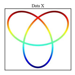
$ $Trifoil Knot は3次元の点の集合であため，この例における SNE では高次元空間(3次元)のデータ $X$ を低次元空間(2次元)のデータ $Y$ へと次元削減します．
低次元空間におけるデータ $Y$ の初期値はランダムに設定しているため，計算するごとに異なる結果が得られます．

以下がクラスタリング結果となります．
クラスタリング結果を見ると，高次元空間のデータの近傍性が低次元空間でもうまく再現されていることが確認できます．

計算過程	クラスタリング結果

3.3 t-SNE の実装

$ $次に t-SNE の実装例を示します．
$ $ほとんどSNE の実装と同じになりますが，低次元空間での近傍関数がスチューデントの $t$ 分布となり，$t$ 分布の自由度 $\nu$ を設定できるようにしてあります．

class tSNE(SNEbase):
    # t-distributed Stochastic Neighbor Embedding

    def __init__(self):
        super(tSNE, self).__init__()

    # 以下のデコレータ(@profile)は line_profiler で実行速度を計測するためのもの
    # use like "kernprof -l -v test.py" on terminal
    # @profile
    def iteration(self, eta, alpha, exaggeration, nu=False):
        # Variables
        # eta : (float) learning rate 勾配降下法の学習率
        # alpha : (float) 勾配降下法(モーメンタム法)におけるモーメント
        # exaggeration : (float) early_exaggeration クラス間の距離を広げるためのトリック
        # nu : (float) t分布の自由度（指定しない時は通常のt-SNEと同じくnu=1.0として計算される）

        self.step += 1

        # 距離Dyを計算
        Ysq = np.sum(np.square(self.Y), axis=1)
        Dy = (Ysq.reshape((self.n,1)) + Ysq) - 2 * self.Y@self.Y.T
        if nu:
            # t-SNE with arbitrary degree of freedom
            # see "Heavy-tailed kernels reveal a finer cluster structure in t-SNE visualisations"
            nu_inv = 1.0/nu
            Dyy = 1.0/(1.0+Dy*nu_inv)
            Dy = np.power(Dyy, 0.5*(nu+1.0))
        else:
            Dy = 1.0/(1.0+Dy)
            Dyy = Dy
        Dy[range(self.n),range(self.n)] = 0.0

        # Q を計算
        # ここでErrorが出る時は学習率を下げてみる
        if self.isSymmetric:
            Q = Dy * (1.0 / np.sum(Dy))
        else:
            Q = Dy / np.sum(Dy, axis=1).reshape((self.n,1))
        Q = np.maximum(Q, 1e-20)
        self.Q = Q

        # exageration(early_exaggeration)はクラス間の距離を広げるらしい
        # DyPQは勾配を計算するための前計算
        DyPQ = Dyy * (exaggeration*self.P - Q)

        # 勾配の計算(slower)
        # grad = []
        # for k in range(self.n):
        #     grad.append( DyPQ[k] @ (self.Y[k]-self.Y) )
        # grad = np.array(grad)

        # 勾配の計算(faster)
        DyPQY1 = np.sum(DyPQ,axis=1).reshape((self.n,1))*self.Y
        DyPQY2 = DyPQ@self.Y
        grad = DyPQY1 - DyPQY2

        # 収束度合いは勾配のノルムで評価(scikit-learnを参考)
        error = np.linalg.norm(grad)

        inc = grad*self.dY < 0.0
        dec = np.logical_not(inc)
        self.gain[inc] = 0.2 + self.gain[inc]
        self.gain[dec] = 0.8 * self.gain[dec]
        self.gain = np.maximum(self.gain, 0.01)

        # SymmetricバージョンとAssymmetricバージョンでetaのスケールを変化させる
        eta = [0.001*eta, eta][self.isSymmetric]

        # update量を計算
        self.dY = alpha*self.dY - eta*self.gain*grad

        # アップデートしてYの平均を0にする（平均を0にした方がエラーになりにくい）
        newY = self.Y + self.dY
        self.Y = newY - np.mean(newY,axis=0)

        return error

$ $上記プログラムないでは，以下のように $t$ 分布の自由度 $\nu$ が 1 の時とそうでない時とで場合分けしています．これは自由度 $\nu$ が 1 の時に比較的計算負荷の大きな np.power() 関数が実行されないようにするためです．

if nu:
    nu_inv = 1.0/nu
    Dyy = 1.0/(1.0+Dy*nu_inv)
    Dy = np.power(Dyy, 0.5*(nu+1.0))
else:
    Dy = 1.0/(1.0+Dy)
    Dyy = Dy

使用例

SNE の時と同じく Trifoil Knot を用いたクラスタリング結果を示します．

以下がクラスタリング結果となります．
$ $$t$-SNE においても，高次元空間のデータの近傍性が低次元空間でもうまく再現されていることが確認できます．

計算過程	クラスタリング結果

3.4 Kernel t-SNE の実装

$ $ここでは Kernel $t$-SNE の実装例を示しています．
Kernel_tSNE クラスは tSNE クラスを継承しています．

try:
    import SNE_kernels as kf
except ModuleNotFoundError:
    kf = False
    print("Module 'SNE_kernels' not found")

class Kernel_tSNE(tSNE):
    # Kernel t-distributed Stochastic Neighbor Embedding

    def __init__(self):
        if not kf:
            raise ModuleNotFoundError("Module 'SNE_kernels' not found")
        super(Kernel_tSNE, self).__init__()

    def fit(self, Xtes, kernel, kernelparam={}):
        if self._Xinit=='pca':
            Xtes = pca(Xtes, self.m).real
        else:
            if self._isXnormalized:
                Xtes = Xtes/np.sum(Xtes, axis=0)
            if self._isXstandardized:
                mean = np.mean(Xtes, axis=0)
                stddev = np.sqrt(np.var(Xtes, axis=0))
                mask = (stddev != 0.0)
                Xtes = (Xtes[:,mask] - mean[mask])/stddev[mask]

        kparam, Ktra = kernel(self.X, self.X, **kernelparam)
        Ktra = Ktra/np.sum(Ktra, axis=1).reshape((self.n,1))
        A = np.linalg.inv(Ktra) @ self.Y

        kparam, Ktes = kernel(Xtes, self.X, **kernelparam)
        Ktes = Ktes/np.sum(Ktes, axis=1).reshape((len(Xtes),1))

        Ytes = Ktes @ A
        return Ytes

$ $上記の Kernel $t$-SNE は理論通りの実装となっているので説明は省略します．
上記プログラム中で読み込んでいる SNE_kernels モジュール内には以下のようにカーネル関数が定義されています．

カーネル関数

def polynomial(X1,X2,a=0.0,c=1.0,p=3):
    """
    polynomial kernel
    X1, X2  : input matrix
    a, c, p : hyper parameter
    f = (a + c*x1@x2)^p
    """
    params = [['kernel','polynomial'], ['a',a], ['c',c], ['p',p]]
    return params,  np.power(c * X1 @ X2.T + a, p)


def gaussian(X1,X2,a=1.0,c=1.0):
    """
    gaussian kernel
    radial basis function
    X1, X2 : input matrix
    a      : hyper parameter
    c      : parameter
    f = c*exp(-a*|x1-x2|^2)
    """
    params = [['kernel','gaussian'], ['a',a], ['c',c]]
    mat = [[norm(x1-x2)**2 for x2 in X2] for x1 in X1]
    mat = np.array(mat).astype(dtype=np.float32)
    return params,  c*np.exp( -a * mat )

使用例

ここでは手書きの文字データを使用した例を示します．
学習データ，テストデータともにデータ数は 600 としてあります．
データは Optical Recognition of Handwritten Digits Data Set を使用しています．

$ $学習用データを $t$-SNE でクラスタリングした結果が以下になります．

クラスタリング前	クラスタリング後

上記の学習結果を用いてテストデータを分類した結果が以下となります．
丸いプロット点(●)が学習データのクラスタリング結果で，星マークのプロット点(★)がテストデータの分類結果を表しています．
カーネル関数には，ガウスカーネルと多項式カーネルを用いており，ハイパーパラメータは手動で設定しました．

多項式カーネル (Polynomial)	ガウスカーネル (Gaussian)

多項式カーネルを用いた分類ではテストデータをうまく分類できたとは言い難いですが，ガウスカーネルの方ではそこそこ上手く分類できていると言っても良さそうですね．
$ $今回はハイパーパラメータの自動チューニングや分類精度の検証などはできませんでしたが，Kernel $t$-SNE を用いるとデータの分類ができることが確認できました．

4. おまけ

4.1 おまけ1 : プログラム一覧

本記事内で用いたプログラム一式を示します．
（※ 展開すると長いプログラムが表示されます）

SNE.py

SNE.py

import numpy as np
old_setting = np.seterr(divide='raise', over='raise', invalid='raise')

try:
    import SNE_kernels as kf
except ModuleNotFoundError:
    kf = False
    print("Module 'SNE_kernels' not found")


# references
# Stochastic Neighbor Embedding, Geoffrey Hinton and Sam Roweis
# Visualizing Data using t-SNE, Laurens van der Maaten, Geoffrey Hinton
# Barnes-Hut-SNE, Laurens van der Maaten
# Accelerating t-SNE using Tree-Based Algorithms, Laurens van der Maaten
# Stochastic Neighbor Embedding, Geoffrey Hinton and Sam Roweis, 
# Heavy-tailed kernels reveal a finer cluster structure in t-SNE visualisations,Dmitry Kobak,George Linderman ,Stefan Steinerberger,Yuval Kluger,Philipp Berens
# Parametric nonlinear dimensionality reduction using kernel t-SNE, Andrej Gisbrecht, z2Alexander Schulz, Barbara Hammer
# TimeCluster: dimension reduction applied to temporal data for visual analytics, Mohammed Ali et.al.
# https://github.com/scikit-learn/scikit-learn/blob/master/sklearn/manifold/_t_sne.py
# https://github.com/scikit-learn/scikit-learn/blob/master/sklearn/manifold/_utils.pyx
# https://distill.pub/2016/misread-tsne/
# http://yusuke-ujitoko.hatenablog.com/entry/2017/05/07/200022



def _binary_search_perplexity(X, perplexity):

    n = len(X)
    Xsq = np.sum(np.square(X), axis=1)
    Dx = (Xsq.reshape((n,1)) + Xsq) - 2 * np.dot(X, X.T)

    maxiter = 200
    eps = 1.0e-10
    beta = np.full(n, 1.0)
    beta_max = np.full(n, np.inf)
    beta_min = np.full(n, -np.inf)
    logPerp = np.log(perplexity)

    for k in range(1,maxiter+1):
        P = np.exp(-Dx*beta.reshape((n,1)))
        P[range(n),range(n)] = 0.0
        P_sum = np.sum(P, axis=1)
        P_sum = np.maximum(P_sum, 1.0e-10)

        # 対数の底を2とする．2^entropy is perplexity
        # >> Perp(pi) = 2^SUMj{pij*log2(pij)}
        # logPerp = np.log2(perplexity)
        # P = P/P_sum.reshape((n,1))
        # H = -np.sum(P*np.log2(P), axis=1)

        # 対数の底をeとする．e^entropy is perplexity
        # >> Perp(pi) = e^SUMj{pij*loge(pij)}
        # logPerp = np.log(perplexity)
        H = np.log(P_sum) + beta*np.sum(Dx*P, axis=1)/P_sum
        P = P/P_sum.reshape((n,1))

        # residual
        diff = H - logPerp

        error = np.abs(diff).max()
        # print('error : ', error)

        if error < eps:
            # print('Binary search of Sigma^2 finished')
            # print('iteration count =', k)
            P = np.maximum(P, np.finfo(np.double).eps)
            P[range(n),range(n)] = 0.0
            perps = np.exp(-np.sum(P*np.log(P+np.identity(n)), axis=1))
            print('Max perplexity is', np.max(perps))
            print('Min perplexity is', np.min(perps))
            print('Average perplexity is', np.mean(perps))
            return P

        # 2分探索
        posMask = diff>0.0
        negMask = np.logical_not(posMask)

        beta_min[posMask] = beta[posMask]
        beta_max[negMask] = beta[negMask]

        maxInfMask = beta_max==np.inf
        mask = posMask*maxInfMask
        beta[mask] = 2.0*beta[mask]
        mask = posMask*np.logical_not(maxInfMask)
        beta[mask] = 0.5*(beta[mask]+beta_max[mask])

        minInfMask = beta_min==-np.inf
        mask = negMask*minInfMask
        beta[mask] = 0.5*beta[mask]
        mask = negMask*np.logical_not(minInfMask)
        beta[mask] = 0.5*(beta[mask]+beta_min[mask])

    raise ValueError("Max iteration over count={}".format(k+1))
    return



def pca(X, embed_dim):
    X = np.array(X)
    (n, d) = X.shape
    X = X - np.mean(X, axis=0)
    (l, M) = np.linalg.eig(X.T@X)
    M = M[:,l>0.0]
    l = l[l>0.0]
    Y = np.dot(X, M[:,:embed_dim])
    return Y



######################################################################
######################################################################
class SNEbase:
    def __init__(self):
        # n = number of data
        # m = dimension of data
        # s = dimension of Y
        # Xoriginal : (np.ndarray) 元のinputデータ行列
        # X : (np.ndarray) (n X m) 計算に使用するデータ行列
        # Y : (np.ndarray) (n X s) SNEで低次元化された行列 (次元sは通常2に設定される)
        # dY : (np.ndarray) (n X s)updating value of Y
        # P : (np.ndarray) (n X n) 特徴空間での確率 P=P(X)
        # Q : (np.ndarray) (n X n) 低次元化後の空間での確率 Q=Q(Y)
        # gain : (np.ndarray) (n X s) (収束性を改善するためのゲイン) gain for gradient of KL Divergence
        # isSymmetric : (bool) 確率Pを対称化するか否か　if use symmetric version
        # step : (integer) ステップ

        self.Xoriginal = None
        self.X = None
        self.Y = None
        self.dY = None
        self.P = None
        self.Q = None
        self.gain = None
        self.isSymmetric = True
        self.n = 0
        self.m = 0
        self.step = 0

        self._Xinit = None
        self._isXnormalized = False
        self._isXstandardized = False


    def setData(self, X, init='pca', embed_dim=2, normalize=False, standardize=False):
        self.Xoriginal  = np.array(X, dtype='float')
        self.X = np.array(X, dtype='float')

        self._Xinit = init
        self._isXnormalized = normalize
        self._isXstandardized = standardize

        if init=='pca':
            print('embedding X with PCA')
            self.X = pca(X, embed_dim).real
            self.n, self.m = self.X.shape
            print('setData() OK.')
            return

        if normalize:
            self.X = self.X/np.sum(self.X, axis=0)

        if standardize:
            mean = np.mean(self.X, axis=0)
            stddev = np.sqrt(np.var(self.X, axis=0))
            mask = (stddev != 0.0)
            self.X = (self.X[:,mask] - mean[mask])/stddev[mask]

        self.n, self.m = self.X.shape
        print('setData() OK.')
        return


    def initialize(self, perplexity=30, n_components=2, initY='pca', isSymmetric=True):
        self.step = 0
        self.isSymmetric = isSymmetric

        # Yの初期化
        if isinstance(initY,np.ndarray):
            if not (len(initY)==self.n):
                raise ValueError("initial Y must have the same number of vector as X")
            self.Y = initY
        elif initY=='random':
            self.Y = 1.0e-4 * np.random.randn(self.n, n_components)
        elif initY=='pca':
            self.Y = pca(self.Xoriginal, n_components).real
        elif initY=='round':
            if not n_components==2:
                raise ValueError("'n_components' must be 2 when initialization method initY='round'")
            theta = np.linspace(0,2*np.pi,self.n, endpoint=False)
            Y = [np.cos(theta), np.sin(theta)]
            self.Y = 1.0e-4 * np.array(Y).T
        else:
            raise ValueError("Select initialization method 'initY'")

        # dY : Yのupdate量
        self.dY = np.zeros((self.n,n_components))
        self.gain = np.full((self.n,n_components),1.0)

        # Pを計算(Gaussianのprecisionは2分探索)
        self.P = _binary_search_perplexity(self.X, perplexity)
        if self.isSymmetric:
            self.P = self.P + self.P.T
            self.P = self.P/np.sum(self.P)
        self.P = np.maximum(self.P, np.finfo(np.double).eps)
        return


    def get_costFunction(self):
        # Cost関数を計算
        return np.sum(self.P * np.log(self.P / self.Q))



######################################################################
######################################################################
class SNE(SNEbase):
    # Stochastic Neighbor Embedding

    def __init__(self):
        super(SNE, self).__init__()

    # 以下のデコレータ(@profile)は line_profiler で実行速度を計測するためのもの
    # use like "kernprof -l -v test.py" on terminal
    # @profile
    def iteration(self, eta, alpha, exaggeration):
        # Variables
        # eta : (float) learning rate 勾配降下法の学習率
        # alpha : (float) 勾配降下法(モーメンタム法)におけるモーメント
        # exaggeration : (float) early_exaggeration クラス間の距離を広げるためのトリック

        self.step += 1

        # 距離Dyを計算
        Ysq = np.sum(np.square(self.Y), axis=1)
        Dy = (Ysq.reshape((self.n,1)) + Ysq) - 2*self.Y@self.Y.T
        Dy[range(self.n),range(self.n)] = 0.0

        # Q を計算
        Q = np.exp(-Dy)
        Q[range(self.n),range(self.n)] = 0.0
        # ここでErrorが出る時は学習率を下げてみる
        if self.isSymmetric:
            Q = Q * (1.0 / np.sum(Q))
        else:
            Q = Q / np.sum(Q, axis=1).reshape((self.n,1))
        Q = np.maximum(Q, 1e-20)
        self.Q = Q

        # exageration(early_exaggeration)はクラス間の距離を広げるらしい
        # PQは勾配を計算するための前計算
        PQ = exaggeration*self.P - Q
        PQ = PQ+PQ.T

        # 勾配の計算(slower)
        # grad = []
        # for k in range(self.n):
        #     grad.append( PQ[k] @ (self.Y[k]-self.Y) )
        # grad = np.array(grad)

        # 勾配の計算(faster)
        PQY1 = np.sum(PQ,axis=1).reshape((self.n,1))*self.Y
        PQY2 = PQ@self.Y
        grad = PQY1 - PQY2

        # 収束度合いは勾配のノルムで評価(scikit-learnを参考)
        error = np.linalg.norm(grad)

        inc = grad*self.dY < 0.0
        dec = np.logical_not(inc)
        self.gain[inc] = 0.2 + self.gain[inc]
        self.gain[dec] = 0.8 * self.gain[dec]
        self.gain = np.maximum(self.gain, 0.01)

        # SymmetricバージョンとAssymmetricバージョンでetaのスケールを変化させる
        eta = [0.001*eta, eta][self.isSymmetric]

        # update量を計算
        self.dY = alpha*self.dY - eta*self.gain*grad

        # アップデートしてYの平均を0にする（平均を0にした方がエラーになりにくい）
        newY = self.Y + self.dY
        self.Y = newY - np.mean(newY,axis=0)

        return error



######################################################################
######################################################################
class tSNE(SNEbase):
    # t-distributed Stochastic Neighbor Embedding

    def __init__(self):
        super(tSNE, self).__init__()

    # 以下のデコレータ(@profile)は line_profiler で実行速度を計測するためのもの
    # use like "kernprof -l -v test.py" on terminal
    # @profile
    def iteration(self, eta, alpha, exaggeration, nu=False):
        # Variables
        # eta : (float) learning rate 勾配降下法の学習率
        # alpha : (float) 勾配降下法(モーメンタム法)におけるモーメント
        # exaggeration : (float) early_exaggeration クラス間の距離を広げるためのトリック
        # nu : (float) t分布の自由度（指定しない時は通常のt-SNEと同じくnu=1.0として計算される）

        self.step += 1

        # 距離Dyを計算
        Ysq = np.sum(np.square(self.Y), axis=1)
        Dy = (Ysq.reshape((self.n,1)) + Ysq) - 2 * self.Y@self.Y.T
        if nu:
            # t-SNE with arbitrary degree of freedom
            # see "Heavy-tailed kernels reveal a finer cluster structure in t-SNE visualisations"
            nu_inv = 1.0/nu
            Dyy = 1.0/(1.0+Dy*nu_inv)
            Dy = np.power(Dyy, 0.5*(nu+1.0))
        else:
            Dy = 1.0/(1.0+Dy)
            Dyy = Dy
        Dy[range(self.n),range(self.n)] = 0.0

        # Q を計算
        # ここでErrorが出る時は学習率を下げてみる
        if self.isSymmetric:
            Q = Dy * (1.0 / np.sum(Dy))
        else:
            Q = Dy / np.sum(Dy, axis=1).reshape((self.n,1))
        Q = np.maximum(Q, 1e-20)
        self.Q = Q

        # exageration(early_exaggeration)はクラス間の距離を広げるらしい
        # DyPQは勾配を計算するための前計算
        DyPQ = Dyy * (exaggeration*self.P - Q)

        # 勾配の計算(slower)
        # grad = []
        # for k in range(self.n):
        #     grad.append( DyPQ[k] @ (self.Y[k]-self.Y) )
        # grad = np.array(grad)

        # 勾配の計算(faster)
        DyPQY1 = np.sum(DyPQ,axis=1).reshape((self.n,1))*self.Y
        DyPQY2 = DyPQ@self.Y
        grad = DyPQY1 - DyPQY2

        # 収束度合いは勾配のノルムで評価(scikit-learnを参考)
        error = np.linalg.norm(grad)

        inc = grad*self.dY < 0.0
        dec = np.logical_not(inc)
        self.gain[inc] = 0.2 + self.gain[inc]
        self.gain[dec] = 0.8 * self.gain[dec]
        self.gain = np.maximum(self.gain, 0.01)

        # SymmetricバージョンとAssymmetricバージョンでetaのスケールを変化させる
        eta = [0.001*eta, eta][self.isSymmetric]

        # update量を計算
        self.dY = alpha*self.dY - eta*self.gain*grad

        # アップデートしてYの平均を0にする（平均を0にした方がエラーになりにくい）
        newY = self.Y + self.dY
        self.Y = newY - np.mean(newY,axis=0)

        return error



######################################################################
######################################################################
class Kernel_tSNE(tSNE):
    # Kernel t-distributed Stochastic Neighbor Embedding

    def __init__(self):
        if not kf:
            raise ModuleNotFoundError("Module 'SNE_kernels' not found")
        super(Kernel_tSNE, self).__init__()

    def fit(self, Xtes, kernel, kernelparam={}):
        if self._Xinit=='pca':
            Xtes = pca(Xtes, self.m).real
        else:
            if self._isXnormalized:
                Xtes = Xtes/np.sum(Xtes, axis=0)
            if self._isXstandardized:
                mean = np.mean(Xtes, axis=0)
                stddev = np.sqrt(np.var(Xtes, axis=0))
                mask = (stddev != 0.0)
                Xtes = (Xtes[:,mask] - mean[mask])/stddev[mask]

        kparam, Ktra = kernel(self.X, self.X, **kernelparam)
        Ktra = Ktra/np.sum(Ktra, axis=1).reshape((self.n,1))
        A = np.linalg.inv(Ktra) @ self.Y

        kparam, Ktes = kernel(Xtes, self.X, **kernelparam)
        Ktes = Ktes/np.sum(Ktes, axis=1).reshape((len(Xtes),1))

        Ytes = Ktes @ A
        return Ytes

SNE_kernels.py

SNE_kernels.py

import numpy as np
from numpy.linalg import norm

"""
kernel function list
'@' means inner product

references
http://crsouza.com/2010/03/17/kernel-functions-for-machine-learning-applications/
https://data-flair.training/blogs/svm-kernel-functions/
"""


def linear(X1,X2,a=0.0,c=1.0):
    """
    linear kernel
    X1, X2 : input matrix
    a,c    : hyper parameter
    f = x1@x2 + a
    """
    params = [['kernel','linear'], ['a',a], ['c',c]]
    return params,  c * X1 @ X2.T + a


def polynomial(X1,X2,a=0.0,c=1.0,p=3):
    """
    polynomial kernel
    X1, X2  : input matrix
    a, c, p : hyper parameter
    f = (a + c*x1@x2)^p
    """
    params = [['kernel','polynomial'], ['a',a], ['c',c], ['p',p]]
    return params,  np.power(c * X1 @ X2.T + a, p)


def gaussian(X1,X2,a=1.0,c=1.0):
    """
    gaussian kernel
    radial basis function
    X1, X2 : input matrix
    a      : hyper parameter
    c      : parameter
    f = c*exp(-a*|x1-x2|^2)
    """
    params = [['kernel','gaussian'], ['a',a], ['c',c]]
    mat = [[norm(x1-x2)**2 for x2 in X2] for x1 in X1]
    mat = np.array(mat).astype(dtype=np.float32)
    return params,  c*np.exp( -a * mat )


def exponential(X1,X2,a=1.0,c=1.0):
    """
    exponential kernel
    laplacian kernel
    X1, X2 : input matrix
    a      : hyper parameter
    c      : parameter
    f = c*exp(-a*|x1-x2|)
    """
    params = [['kernel','exponential'], ['a',a], ['c',c]]
    mat = [[norm(x1-x2) for x2 in X2] for x1 in X1]
    mat = np.array(mat).astype(dtype=np.float32)
    return params,  c*np.exp(-a * mat)


def ANOVA(X1,X2,a=1.0,k=1.0,p=1.0):
    """
    ANOVA kernel
    X1, X2  : input matrix
    a, k, p : hyper parameter
    f = SUM(exp(-a*|x1_i^k-x2i^k|^2)^p)
    """
    params = [['kernel','ANOVA'], ['a',a], ['k',k], ['p',p]]
    mat = [[(x1**k-x2**k) for x2 in X2] for x1 in X1]
    mat = np.array(mat).astype(dtype=np.float32)
    return params,  np.sum( np.exp(-a*np.square(mat))**p, axis=2)


def sigmoid(X1,X2,a=0.0,c=1):
    """
    sigmoid kernel
    X1, X2 : input matrix
    a, c   : hyper parameter
    f = tanh(a + c*x1@x2)    
    """
    params = [['kernel','sigmoid'], ['a',a], ['c',c]]
    return params,  np.tanh(c * X1 @ X2.T + a)


def rational_quadratic(X1,X2,a=1.0):
    """
    rational quadratic kernel
    X1, X2 : input matrix
    a      : hyper parameter
    f = 1 - |x1-x2|^2 / (|x1-x2|^2 + a)
    """
    params = [['kernel','rational_quadratic'], ['a',a]]
    mat = [[norm(x1-x2)**2 for x2 in X2] for x1 in X1]
    mat = np.array(mat).astype(dtype=np.float32)
    return params,  1-mat/(mat+a)


def multi_quadratic(X1,X2,a=1.0,c=1.0):
    """
    multi quadratic kernel
    X1, X2 : input matrix
    a, c   : hyper parameter
    f = sqrt( |x1-x2|^2 + a^2 )
    """
    params = [['kernel','multi_quadratic'], ['a',a]]
    mat = [[norm(x1-x2)**2 for x2 in X2] for x1 in X1]
    mat = np.array(mat).astype(dtype=np.float32)
    return params,  np.sqrt(c*mat + a*a)


def inverse_multi_quadratic(X1,X2,a=1.0):
    """
    inverse multi quadratic kernel
    X1, X2 : input matrix
    a      : hyper parameter
    f = 1 / sqrt( |x1-x2|^2 + a^2 )
    """
    params = [['kernel','inverse_multi_quadratic'], ['a',a]]
    mat = [[norm(x1-x2)**2 for x2 in X2] for x1 in X1]
    mat = 1/np.array(mat).astype(dtype=np.float32)
    return params,  mat


def circular(X1,X2,a=1.0):
    """
    cicular kernel
    X1, X2 : input matrix
    a      : hyper parameter
    f = 2/pi * arccos(-|x1-x2|/a) - 2/pi * |x1-x2|/a * sqrt(a-(|x1-x2|/a)^2)
    """
    params = [['kernel','circular'], ['a',a]]
    mat = [[norm(x1-x2)/a for x2 in X2] for x1 in X1]
    mat = np.array(mat).astype(dtype=np.float32)
    mat[mat>1] = 0
    c = 2/np.pi
    return params,  c*np.arccos(-mat) - c*mat*np.sqrt(1-mat*mat)


def triangular(X1,X2,a=1.0):
    """
    triangular kernel
    X1, X2 : input matrix
    a      : hyper parameter
    f = 1 - |x1-x2|/a
    """
    params = [['kernel','triangular'], ['a',a]]
    mat = [[norm(x1-x2)/a for x2 in X2] for x1 in X1]
    mat = np.array(mat).astype(dtype=np.float32)
    mat[mat>1] = 0
    return params,  1 - mat


def spherical(X1,X2,a=1.0):
    """
    spherical kernel
    X1, X2 : input matrix
    a      : hyper parameter
    f = 1 - 3/2 * |x1-x2|/a + 1/2 * (|x1-x2|/a)^3
    """
    params = [['kernel','spherical'], ['a',a]]
    mat = [[norm(x1-x2)/a for x2 in X2] for x1 in X1]
    mat = np.array(mat).astype(dtype=np.float32)
    mat[mat>1] = 0
    return params,  1 - 1.5 * mat + 0.5 * mat*mat*mat


def power(X1,X2,p=1.0):
    """
    power kernel
    X1, X2 : input matrix
    p      : hyper parameter
    f = - |x1-x2|^p
    """
    params = [['kernel','power'], ['p',p]]
    mat = [[-norm(x1-x2)**p for x2 in X2] for x1 in X1]
    mat = np.array(mat).astype(dtype=np.float32)
    return params,  mat


def log(X1,X2,p=1.0):
    """
    log kernel
    X1, X2 : input matrix
    p      : hyper parameter
    f = - log(|x1-x2|^p + 1)
    """
    params = [['kernel','log'], ['p',p]]
    mat = [[norm(x1-x2)**p for x2 in X2] for x1 in X1]
    mat = np.array(mat).astype(dtype=np.float32)
    return params,  -np.log(mat + 1)


def generalized_t_student(X1,X2,p=1.0):
    """
    generalized T-Studente kernel
    X1, X2 : input matrix
    p      : hyper parameter
    f = 1 / (|x1-x2|^p + 1)
    """
    params = [['kernel','generalized_t_student'], ['p',p]]
    mat = [[1/(norm(x1-x2)**p+1) for x2 in X2] for x1 in X1]
    mat = np.array(mat).astype(dtype=np.float32)
    return params,  mat

TrifoilKnot.py

TrifoilKnot.py

import numpy as np
import matplotlib.pyplot as plt
import matplotlib.cm as cm

from SNE import *

plt.rcParams['font.family'] = 'Times New Roman'
plt.rcParams['font.size'] = 14
plt.rcParams['axes.linewidth'] = 1.6

# データ点数
n = 200

phi = np.linspace(0,2*np.pi,num=n,endpoint=False)
x = np.sin(phi)+2*np.sin(2*phi)
y = np.cos(phi)-2*np.cos(2*phi)
z = -np.sin(3*phi)
s = np.abs(((y+3)+2)*10)

X = np.array([x,y,z]).T
c = s

initY = 2*np.random.normal(loc=0,scale=1,size=(len(X),2))

plt.figure(figsize=(4,4), dpi=100)
plt.title('Data X')
plt.scatter(X[:,0], X[:,1], c=c, s=30, cmap='jet')
plt.subplots_adjust(left=0.01, right=0.99, bottom=0.01, top=0.9)
plt.xticks([],[])
plt.yticks([],[])
plt.tight_layout()
plt.savefig('TrifoilKnot_initial.jpg',bbox_bound='tight')
plt.show()

##########################################################
##########################################################

sne = SNE()     # when SNE
# sne = tSNE()    # when tSNE

sne.setData(X, init='pca', embed_dim=50, normalize=False, standardize=False)
sne.initialize(perplexity=20, n_components=2, initY=initY, isSymmetric=True)

# learning rate
eta = 200

maxiter = 200 + 1
nshow_error = 10
nshow_plot = 100
tol = 1.0e-8

saveAnimation = True
Y_history = []
E_history = []
S_history = []
error = 0.0

for i in range(maxiter):

    if saveAnimation:
        Y_history.append(sne.Y)
        E_history.append(error)
        S_history.append(sne.step)

    if not sne.step%nshow_plot:
        plt.close('all')
        plt.figure(figsize=(4,4), dpi=100)
        plt.title('Step = '+str(sne.step))
        plt.scatter(sne.Y[:,0], sne.Y[:,1], c=c, s=30, cmap='jet')
        plt.tight_layout()
        plt.show()

    if sne.step<20:
        alpha = 0.8
    else:
        alpha = 0.4

    if sne.step<60:
        exaggeration = 2.0
    else:
        exaggeration = 1.0

    error = sne.iteration(eta=eta, alpha=alpha, exaggeration=exaggeration)

    if not sne.step%nshow_error:
        print('Step :', sne.step, '\tError :', error)

    # if error < tol:
    #     print('Iteration stopped due to enough convergence!')
    #     break

plt.close('all')
plt.figure(figsize=(4,4), dpi=100)
plt.title('Final Result : Step = '+str(sne.step))
plt.scatter(sne.Y[:,0], sne.Y[:,1], c=c, s=30, cmap='jet')
plt.subplots_adjust(left=0.01, right=0.99, bottom=0.01, top=0.9)
plt.xticks([],[])
plt.yticks([],[])
plt.tight_layout()
plt.savefig('TrifoilKnot_final.jpg',bbox_bound='tight')
plt.show()


if not saveAnimation:
    exit()

try:
    # save animation
    # run on terminal(command prompt if not worked)
    import matplotlib.animation as animation

    fig = plt.figure(figsize=(4,4), dpi=100)

    def animate(n):
        plt.cla()
        plt.title('Step={:04d},  Error={:.3e}'.format(S_history[n], E_history[n]), pad=10)
        plt.subplots_adjust(left=0.01, right=0.99, bottom=0.01, top=0.9)
        plt.scatter(Y_history[n][:,0], Y_history[n][:,1], c=c, s=30, cmap='jet')
        plt.xlim(xmin=-5, xmax=5)
        plt.ylim(ymin=-5, ymax=5)
        plt.xticks([],[])
        plt.yticks([],[])

    anim = animation.FuncAnimation(fig,animate,interval=100,blit=False,frames=len(S_history))
    anim.save('./TrifoilKnot.mp4', writer="ffmpeg")
    plt.close('all')
except UnicodeDecodeError:
    pass

Digits_kernel.py

Digits_kernel.py

from copy import deepcopy

import numpy as np
import matplotlib.pyplot as plt
import matplotlib.cm as cm
from matplotlib.offsetbox import OffsetImage,AnnotationBbox
from SNE import *

plt.rcParams['font.family'] = 'Times New Roman'
plt.rcParams['font.size'] = 14
plt.rcParams['axes.linewidth'] = 1.6

X = []
label = []
f = open('./data/optdigits.tra')
for row in f.readlines():
    line = row.strip().split(',')
    if len(line) < 2:
        break
    X.append(line[:-1])
    label.append(line[-1])
f.close()

n = 600
ntra = 600
Xtes = np.array(X, dtype=np.float)[n:n+ntra]
label_tes = np.array(label, dtype=np.int)[n:n+ntra]
X = np.array(X, dtype=np.float)[:n]
label = np.array(label, dtype=np.int)[:n]
# print(X[0].shape)
# print(np.sqrt(len(X[0])))
# print(X[0])
# img_grey = X[0].reshape((8,8))
# plt.imshow(img_grey, cmap='binary')
# plt.show()
# exit()


cmap = 'hsv'
Ximg = deepcopy(X)
Ximg_norm = Ximg/np.max(Ximg, axis=1).reshape((n,1))
Ximg = Ximg-np.mean(Ximg, axis=1).reshape((n,1))
Ximg = Ximg/np.max(np.abs(Ximg), axis=1).reshape((n,1))
Ximg = (1/20)+0.1*label.reshape((n,1)) + Ximg/20
Ximg = (Ximg-Ximg.min())/(Ximg.max()-Ximg.min())
Ximg = plt.get_cmap(cmap)(Ximg)
Ximg[:,:,3] = np.sqrt(Ximg_norm)
# print(Ximg[0])
# print(Ximg[0].shape)
# plt.imshow(Ximg[0].reshape((8,8,4)), cmap='jet', vmin=0, vmax=1)
# plt.show()
# # exit()


initY = 3*np.random.normal(loc=0,scale=1,size=(len(X),2))

plt.close('all')
plt.figure(figsize=(4,4), dpi=200)
plt.title('Initial State')
for k in range(label.min(),label.max()+1):
    x = initY[label==k,0]
    y = initY[label==k,1]
    plt.plot(x, y, 'o', color=cm.hsv(k/(label.max()+1)), ms=5, label=str(k))
plt.legend(loc='upper left', bbox_to_anchor=(1, 1))
plt.xticks([],[])
plt.yticks([],[])
plt.tight_layout()
plt.savefig('Digits_kernel_initial.jpg',bbox_bound='tight')
plt.show()

##########################################################
##########################################################

sne = Kernel_tSNE()
sne.setData(X, init='', embed_dim=30, normalize=False, standardize=False)
sne.initialize(perplexity=50, n_components=2, initY='pca', isSymmetric=True)

# learning rate
eta = 600

maxiter = 2000
nshow_error = 100
nshow_plot = 200
tol = 1.0e-7

saveAnimation = False
Y_history = []
E_history = []
S_history = []
error = 0.0

for i in range(maxiter):

    if saveAnimation:
        Y_history.append(sne.Y)
        E_history.append(error)
        S_history.append(sne.step)

    if not sne.step%nshow_plot:
        plt.close('all')
        plt.figure(figsize=(4,4), dpi=200)
        ax = plt.subplot()
        plt.title('Step = '+str(sne.step))
        for k in range(label.min(),label.max()+1):
            x = sne.Y[label==k,0]
            y = sne.Y[label==k,1]
            plt.plot(x, y, 'o', color=cm.hsv(k/(label.max()+1)), ms=5, label=str(k), alpha=0.0)
            img_list = Ximg[label==k]
            for s in range(len(img_list)):
                arr_img = img_list[s].reshape((8,8,4))
                imagebox = OffsetImage(arr_img, zoom=1.0, cmap=cmap)
                imagebox.image.axes = ax
                ab = AnnotationBbox(imagebox, (x[s], y[s]), xycoords='data', frameon=False)
                ax.add_artist(ab)
        plt.xticks([],[])
        plt.yticks([],[])
        # plt.legend(loc='upper left', bbox_to_anchor=(1, 1))
        plt.tight_layout()

        if sne.step==0:
            plt.savefig('Digits_kernel_initial2.jpg',bbox_bound='tight')

        plt.show()

    if sne.step<300:
        alpha = 0.8
    else:
        alpha = 0.4

    if sne.step<600:
        exaggeration = 2.0
    else:
        exaggeration = 1.0

    error = sne.iteration(eta=eta, alpha=alpha, exaggeration=exaggeration, nu=0.5)

    if not sne.step%nshow_error:
        print('Step :', sne.step, '\tError :', error)

    if error < tol:
        print('Iteration stopped due to enough convergence!')
        break


plt.close('all')
plt.figure(figsize=(5.5,4), dpi=200)
plt.title('Final Result : Step = '+str(sne.step))
for k in range(label.min(),label.max()+1):
    x = sne.Y[label==k,0]
    y = sne.Y[label==k,1]
    plt.plot(x, y, 'o', color=cm.hsv(k/(label.max()+1)), ms=5, label=str(k))
plt.legend(loc='upper left', bbox_to_anchor=(1, 1))
plt.xticks([],[])
plt.yticks([],[])
plt.tight_layout()
plt.savefig('Digits_kernel_final.jpg',bbox_bound='tight')
plt.show()

plt.close('all')
plt.figure(figsize=(4,4), dpi=200)
ax = plt.subplot()
plt.title('Final Result : Step = '+str(sne.step))
for k in range(label.min(),label.max()+1):
    x = sne.Y[label==k,0]
    y = sne.Y[label==k,1]
    plt.plot(x, y, 'o', color=cm.hsv(k/(label.max()+1)), ms=5, label=str(k), alpha=0.0)
    img_list = Ximg[label==k]
    for s in range(len(img_list)):
        arr_img = img_list[s].reshape((8,8,4))
        imagebox = OffsetImage(arr_img, zoom=1.0, cmap=cmap)
        imagebox.image.axes = ax
        ab = AnnotationBbox(imagebox, (x[s], y[s]), xycoords='data', frameon=False)
        ax.add_artist(ab)
plt.xticks([],[])
plt.yticks([],[])
# plt.legend(loc='upper left', bbox_to_anchor=(1, 1))
plt.tight_layout()
plt.savefig('Demo11_Digits_kernel_final2.jpg',bbox_bound='tight')


from SNE_kernels import *
# Try following
# kernel, kernelparam = linear, {'a':1.0, 'c':0.01}
# kernel, kernelparam = polynomial, {'p':3, 'a':1, 'c':0.1}
kernel, kernelparam = gaussian, {'a':0.01, 'c':1.0}
# kernel, kernelparam = exponential, {'a':3.0, 'c':1.0}
# kernel, kernelparam = ANOVA, {'a':0.1, 'k':1.0, 'p':1.0}
# kernel, kernelparam = sigmoid, {'a':1.0, 'c':0.01}
# kernel, kernelparam = rational_quadratic, {'a':1.0}
# kernel, kernelparam = power, {'p':5.0}
# kernel, kernelparam = log, {'p':1.0}
# kernel, kernelparam = generalized_t_student, {'p':1.0}



kernel, kernelparam = gaussian, {'a':0.01, 'c':1.0}
Ytes = sne.fit(Xtes, kernel=kernel, kernelparam=kernelparam)
plt.close('all')
plt.figure(figsize=(5.5,4), dpi=200)
plt.title('Fit Result')
for k in range(label.min(),label.max()+1):
    x = sne.Y[label==k,0]
    y = sne.Y[label==k,1]
    plt.plot(x, y, 'o', color=cm.hsv(k/(label.max()+1)), ms=5, label=str(k))
for k in range(label_tes.min(),label_tes.max()+1):
    x = Ytes[label_tes==k,0]
    y = Ytes[label_tes==k,1]
    plt.plot(x, y, '*', color=cm.hsv(k/(label.max()+1)), ms=5,
        markeredgewidth=0.2, markeredgecolor='black')
plt.legend(loc='upper left', bbox_to_anchor=(1, 1))
plt.xticks([],[])
plt.yticks([],[])
plt.tight_layout()
plt.savefig('Digits_kernel_mapped.jpg',bbox_bound='tight')
plt.show()


if not saveAnimation:
    exit()

try:
    # save animation
    # run on terminal(command prompt if not worked)
    import matplotlib.animation as animation

    fig = plt.figure(figsize=(4,4), dpi=100)
    ax = plt.subplot()
    def animate(n):
        print(n)
        plt.cla()
        plt.title('Step={:04d},  Error={:.3e}'.format(S_history[n], E_history[n]), pad=10)
        for k in range(label.min(),label.max()+1):
            x = Y_history[n][label==k,0]
            y = Y_history[n][label==k,1]
            plt.plot(x, y, 'o', color=cm.hsv(k/(label.max()+1)), ms=5, label=str(k), alpha=0.0)
            img_list = Ximg[label==k]
            for s in range(len(img_list)):
                arr_img = img_list[s].reshape((8,8,4))
                imagebox = OffsetImage(arr_img, zoom=1.0, cmap=cmap)
                imagebox.image.axes = ax
                ab = AnnotationBbox(imagebox, (x[s], y[s]), xycoords='data', frameon=False)
                ax.add_artist(ab)
        # plt.xlim(xmin=-18, xmax=10)
        # plt.ylim(ymin=-18, ymax=10)
        plt.xticks([],[])
        plt.yticks([],[])

    anim = animation.FuncAnimation(fig,animate,interval=100,blit=False,frames=len(S_history))
    anim.save('./Digits.mp4', writer="ffmpeg")
    plt.close('all')
except UnicodeDecodeError:
    pass

Digits_kernel.py 中で使用しているデータ optdigits.tra は Optical Recognition of Handwritten Digits Data Set からダウンロードできます．

4.2 おまけ2 : scikit-learnによるt-SNE

$ $scikit-learnにも$t$-SNEは実装されています．
https://scikit-learn.org/stable/modules/generated/sklearn.manifold.TSNE.html

$ $以下に，scikit-learn における $t$-SNE の実装例を示します．

scikit-learnによるt-SNEの実装例(TrifoilKnot)

scikit-learnによるt-SNEの実装例(TrifoilKnot)

import numpy as np
import matplotlib.pyplot as plt
from sklearn.manifold import TSNE

# データ点数
n = 200

phi = np.linspace(0,2*np.pi,num=n,endpoint=False)
x = np.sin(phi)+2*np.sin(2*phi)
y = np.cos(phi)-2*np.cos(2*phi)
z = -np.sin(3*phi)
s = np.abs(((y+3)+2)*10)

X = np.array([x,y,z]).T
c = s

print('In high-dimensional space : ', X.shape)

X_reduced = TSNE(n_components=2, random_state=0).fit_transform(X)

print('In low-dimensional space : ', X_reduced.shape)

plt.scatter(X_reduced[:, 0], X_reduced[:, 1], c=c)
plt.colorbar()
plt.show()

実行結果

scikit-learnによるt-SNEの実装例(digits)

scikit-learnによるt-SNEの実装例(digits)

import matplotlib.pyplot as plt
from sklearn import datasets
from sklearn.manifold import TSNE

digits = datasets.load_digits()

print('In high-dimensional space : ', digits.target.shape)

X_reduced = TSNE(n_components=2, random_state=0).fit_transform(digits.data)

print('In low-dimensional space : ', X_reduced.shape)

plt.scatter(X_reduced[:, 0], X_reduced[:, 1], c=digits.target)
plt.colorbar()
plt.show()

実行結果

おわりに

本記事では下記項目について解説をしました．

• SNE の理論と実装
• $t$-SNE の理論と実装
• Kernel $t$-SNE の理論と実装

今回，SNE の実装を行うにあたっていろいろなサイトや論文を参考にしましたがプログラムの実装方針を示してくれているものは非常に限られていることが分かりました．論文中に書かれている数式とプログラムが違っていたりすると私のような初心者では？？？となってしまい，その疑問を解決するのに結構な時間がかかります．また論文などには記載されないがプログラム中では実装されている収束性を改善する計算トリックのようなものも使われていることがわかりました．
こうした点が，クラスタリングをはじめ機械学習手法の実装を難しくしている要因だと思うので，プログラムの実装方針を示してくれる記事が増えるといいなと思います．

$ $本記事では　Kernel $t$-SNE を扱いましたが，似たような手法に UMAP と呼ばれるものがあります．UMAP も次元削減により高次元データを可視化することができます．また，新規に追加されたデータの分類も可能です．
下記に参考リンクを示しておきますので興味のある方は是非読んでみてください．

• UMAP: Uniform Manifold Approximation and Projection for Dimension Reduction
• https://github.com/lmcinnes/umap
• UMAP 論文を読む

参考資料

[1] Stochastic Neighbor Embedding
[2] Visualizing Data using t-SNE
[3] An Analysis of the t-SNE Algorithm for Data Visualization
[4] Learning a Parametric Embedding by Preserving Local Structure
[5] Heavy-Tailed Symmetric Stochastic Neighbor Embedding
[6] Out-of-Sample Kernel Extensions for Nonparametric Dimensionality Reduction
[7] Parametric nonlinear dimensionality reduction using kernel t-SNE
[8] t-SNE
[9] 高次元のデータを可視化するt-SNEの効果的な使い方
[10] t-SNE clearly explained
[11] t-SNEを理解して可視化力を高める