ggplot2のscale_*()関数についてのまとめ

はじめに

ggplot2では、データから、stat_*()関数やgeom_*()関数で基本的なグラフのレイヤーを描き、scale_*()関数で軸の設定をします。
今回は、ggplot2における軸の設定についてまとめます。

目次

• scale_*()
  • scale_x_*(), scale_y_*()：x軸, y軸
    • scale_x_continuous(), scale_y_continuous()：連続値のx軸, y軸
      • 引数name：軸のラベル
      • 引数breaks：軸の目盛り
      • 引数minor_breaks：軸の補助目盛り
      • 引数labels：軸の目盛りのラベル
      • 引数limits：軸の範囲
      • 引数expand：値の範囲の外に拡張される軸の幅
      • 引数trans：軸のスケール変換
      • 引数position：軸の表示場所
      • 引数guide：軸の凡例
        • guide_axis()：軸の凡例を設定する関数
          • 引数n.dodge：軸のラベルを複数列にずらして表示
          • 引数angle：軸のラベルの表示の角度
      • 引数sec.axis：第２軸
    • scale_x_discrete(), scale_y_discrete()：離散値のx軸, y軸
      • 引数name：軸のラベル
      • 引数labels：軸の目盛りのラベル
      • 引数limits：軸の範囲
      • 引数expand：値の範囲の外に拡張される軸の幅
      • 引数position：軸の表示場所
      • 引数guide：軸の凡例
        • guide_axis()：軸の凡例を設定する関数
          • 引数n.dodge：軸のラベルを複数列にずらして表示
          • 引数angle：軸のラベルの表示の角度
    • scale_x_binned(), scale_y_binned()：連続値のx軸, y軸のビン分割
      • 引数name：軸のラベル
      • 引数n.breaks, nice.breaks
      • 引数show.limits
      • 引数breaks：軸の目盛り
      • 引数limits：軸の範囲
      • 引数labels：軸の目盛りのラベル
      • 引数trans：軸のスケール変換
  • scale_color_*(), scale_fill_*(), scale_alpha_*(), scale_size_*(), scale_shape_*(), scale_linetype_*()：color軸, fill軸, alpha軸, shape軸, size軸, linetype軸
    • scale_*_continuous()：連続値のcolor軸など
    • scale_*_binned()：連続値のcolor軸などのビン分割
    • scale_*_discrete()：離散値のcolor軸など
      • 引数name：軸のラベル
      • 引数breaks：軸の目盛り
      • 引数labels：軸の目盛りのラベル
      • 引数limits：軸の範囲
      • 引数trans：軸のスケール変換
      • 引数guide：軸の凡例
        • guide_legend()：凡例を設定する関数
          • 引数reverse：凡例の軸の反転
          • 引数nrow, ncol, byrow：凡例を何行何列に表示するか
          • 引数title, title.position：凡例のタイトル
          • 引数label, label.position：凡例のラベル
        • guide_colorbar()：カラーバーを設定する関数
          • 引数barwidth, barheiht：カラーバーの大きさ
          • 引数ticks, ticks.colour, ticks.linewidth：カラーバーの目盛り
        • guide_bins()
        • guide_coloursteps()
          • 引数even.steps
          • 引数show.limits
          • 引数axis.arrow
    • scale_*_manual()：離散値のcolor軸などの手動設定
      • 引数values：手動設定したい値の指定
    • scale_*_identity()：color軸などのデータの値をそのまま設定
  • scale_color_*(), scale_fill_*()：color軸, fill軸
    • scale_color_gradient(), scale_fill_gradient()：連続値のcolor軸, fill軸
    • scale_color_steps(), scale_fill_steps()：連続値のcolor軸, fill軸のビン分割
    • scale_color_gradient2(), scale_fill_gradient2()：連続値のcolor軸, fill軸
    • scale_color_steps2(), scale_fill_steps2()：連続値のcolor軸, fill軸のビン分割
    • scale_color_gradientn(), scale_fill_gradientn()：連続値のcolor軸, fill軸
    • scale_color_stepsn(), scale_fill_stepsn()：連続値のcolor軸, fill軸のビン分割
    • scale_color_distiller(), scale_fill_distiller()：連続値のcolor軸, fill軸
    • scale_color_fermenter(), scale_fill_fermenter()：連続値のcolor軸, fill軸のビン分割
    • scale_color_continuous(), scale_fill_continuous()：連続値のcolor軸, fill軸
    • scale_color_binned(), scale_fill_binned()：連続値のcolor軸, fill軸のビン分割
    • scale_color_viridis_c(), scale_fill_viridis_c()：連続値のcolor軸, fill軸
    • scale_colour_viridis_b(), scale_fill_viridis_b()：連続値のcolor軸, fill軸のビン分割
    • scale_color_brewer(), scale_fill_brewer()：離散値のcolor軸, fill軸
    • scale_color_grey(), scale_fill_grey()：離散値のcolor軸, fill軸
    • scale_color_hue(), scale_fill_hue()：離散値のcolor軸, fill軸
    • scale_color_discrete(), scale_fill_discrete()：離散値のcolor軸, fill軸
    • scale_color_viridis_d(), scale_fill_viridis_d()：離散値のcolor軸, fill軸
  • scale_shape_*()：shape軸
    • scale_shape_discrete(), scale_shape_binned()：離散値のshape軸, 連続値のshape軸のビン分割
      • 引数solid：shapeの塗りつぶし
• まとめ
• 参考文献

R

library(tidyverse)

scale_*()

ggplot2では、軸の設定はscale_*()関数で行います。

scale_x_*(), scale_y_*()：x軸, y軸

x軸, y軸の設定をします。
連続値のときはscale_*_continuous()、離散値のときはscale_*_discrete()を使います。また、連続値をビン分割する場合はscale_*_binned()を使います。

• scale_*_continuous()：連続（continuous）値の場合
• scale_*_discrete()：離散（discrete）値の場合
• scale_*_binned()：連続（continuous）値の場合（ビン分割）

scale_x_continuous(), scale_y_continuous()：連続値のx軸, y軸

x軸, y軸が連続値の場合、scale_x_continuous(), scale_y_continuous()で軸の設定を調整します。

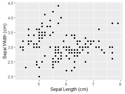
引数name：軸のラベル

nameで軸のラベルに表示される文字列を設定できます。
xlab(), ylab()でも設定できます。また、labs(x = ..., y = ...)でも設定できます。

R

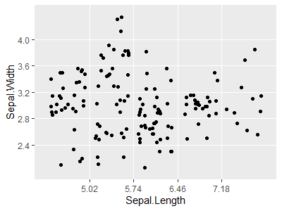
ggplot(data = iris, aes(x = Sepal.Length, y = Sepal.Width)) +
  geom_point() +
  scale_x_continuous(name = "Sepal Length (cm)") +
  scale_y_continuous(name = "Sepal Width (cm)")
ggplot(data = iris, aes(x = Sepal.Length, y = Sepal.Width)) +
  geom_point() +
  xlab("Sepal Length (cm)") +
  ylab("Sepal Width (cm)")
ggplot(data = iris, aes(x = Sepal.Length, y = Sepal.Width)) +
  geom_point() +
  labs(x = "Sepal Length (cm)", y = "Sepal Width (cm)")

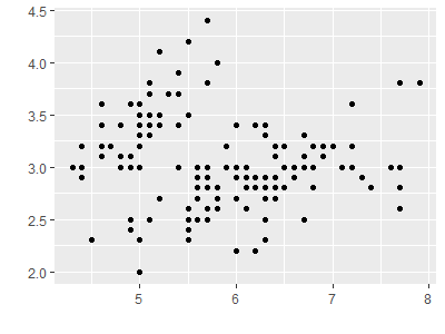
ggplot(data = iris, aes(x = Sepal.Length, y = Sepal.Width)) +
  geom_point() +
  scale_x_continuous(name = "") +
  scale_y_continuous(name = "")
ggplot(data = iris, aes(x = Sepal.Length, y = Sepal.Width)) +
  geom_point() +
  xlab("") +
  ylab("")
ggplot(data = iris, aes(x = Sepal.Length, y = Sepal.Width)) +
  geom_point() +
  labs(x = "", y = "")

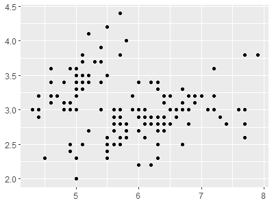
NULLにすると軸のラベルの表示自体がなくなります。

R

ggplot(data = iris, aes(x = Sepal.Length, y = Sepal.Width)) +
  geom_point() +
  scale_x_continuous(name = NULL) +
  scale_y_continuous(name = NULL)
ggplot(data = iris, aes(x = Sepal.Length, y = Sepal.Width)) +
  geom_point() +
  xlab(label = NULL) +
  ylab(label = NULL)
ggplot(data = iris, aes(x = Sepal.Length, y = Sepal.Width)) +
  geom_point() +
  labs(x = NULL, y = NULL)

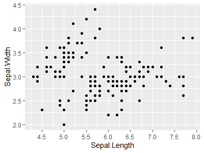
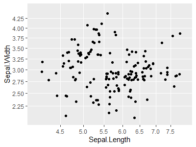
なお、デフォルトではname = waiver()で、軸の変数名がそのまま表示されます。

R

ggplot(data = iris, aes(x = Sepal.Length, y = Sepal.Width)) +
  geom_point()
ggplot(data = iris, aes(x = Sepal.Length, y = Sepal.Width)) +
  geom_point() +
  scale_x_continuous() +
  scale_y_continuous()
ggplot(data = iris, aes(x = Sepal.Length, y = Sepal.Width)) +
  geom_point() +
  scale_x_continuous(name = waiver()) +  # デフォルト
  scale_y_continuous(name = waiver())    # デフォルト

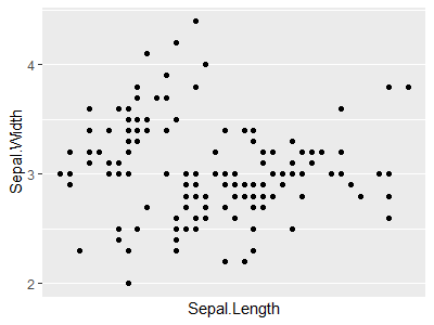
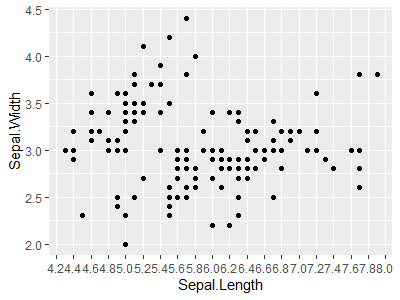
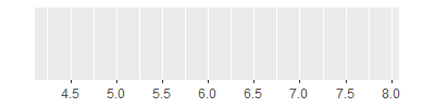
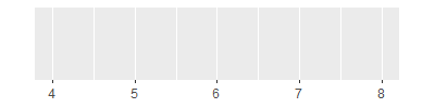
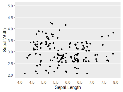
引数breaks：軸の目盛り

breaksで軸の目盛りを設定できます。

R

ggplot(data = iris, aes(x = Sepal.Length, y = Sepal.Width)) +
  geom_point() +
  scale_x_continuous(breaks = 4:8) +
  scale_y_continuous(breaks = 2:5)

seq(4, 8, by = 0.5)
# [1] 4.0 4.5 5.0 5.5 6.0 6.5 7.0 7.5 8.0
seq(2, 5, by = 0.5)
# [1] 2.0 2.5 3.0 3.5 4.0 4.5 5.0
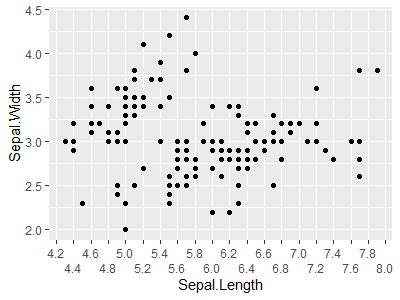
ggplot(data = iris, aes(x = Sepal.Length, y = Sepal.Width)) +
  geom_point() +
  scale_x_continuous(breaks = seq(4, 8, by = 0.5)) +
  scale_y_continuous(breaks = seq(2, 5, by = 0.5))

NULLとすると軸の目盛りの表示がなくなります。

R

ggplot(data = iris, aes(x = Sepal.Length, y = Sepal.Width)) +
  geom_point() +
  scale_x_continuous(breaks = NULL) +
  scale_y_continuous(breaks = 2:5)

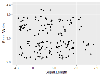
なお、breaksは等間隔でなくても構いません。

R

ggplot(data = iris, aes(x = Sepal.Length, y = Sepal.Width)) +
  geom_point() +
  scale_x_continuous(breaks = c(4:8, range(iris$Sepal.Length)),
                     minor_breaks = NULL,
                     limits = c(4, 8)) +
  scale_y_continuous(breaks = c(2:5, range(iris$Sepal.Width)),
                     minor_breaks = NULL,
                     limits = c(2, 5))

c(4:8, range(iris$Sepal.Length))
# [1] 4.0 5.0 6.0 7.0 8.0 4.3 7.9
c(2:5, range(iris$Sepal.Width))
# [1] 2.0 3.0 4.0 5.0 2.0 4.4

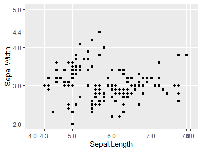
注）わかりやすいようにminor_breaks = NULLで補助目盛りを削除し、limitsで軸の範囲を指定してあります（minor_breaks、limitsについては以下の項を参照。）。

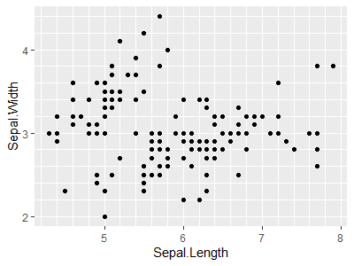
引数minor_breaks：軸の補助目盛り

minor_breaksで軸の補助目盛り（軸の目盛りの間の目盛り）を設定できます。

R

ggplot(data = iris, aes(x = Sepal.Length, y = Sepal.Width)) +
  geom_point() +
  scale_x_continuous(breaks = 4:8, minor_breaks = seq(4, 8, by = 0.2)) +
  scale_y_continuous(breaks = 2:5, minor_breaks = seq(2, 5, by = 0.2))

ggplot(data = iris, aes(x = Sepal.Length, y = Sepal.Width)) +
  geom_point() +
  scale_x_continuous(breaks = 4:8, minor_breaks = NULL) +
  scale_y_continuous(breaks = 2:5, minor_breaks = NULL)

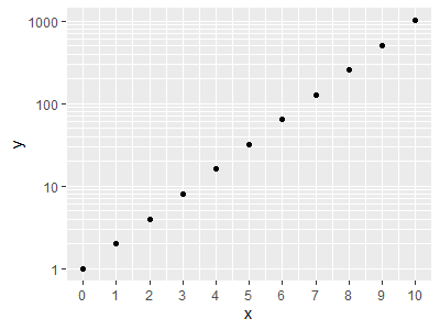
minor_breaksも等間隔でなくても構いません。

R

ggplot(data = data.frame(x = 0:10, y = 2^(0:10)), aes(x = x, y = y)) +
  geom_point() +
  scale_x_continuous(trans = "identity",
                     breaks = 0:10) +
  scale_y_continuous(trans = "log10",
                     breaks = 10^(0:3),
                     minor_breaks = unique(as.numeric(1:10 %o% 10 ^ (0:3))),
                     labels = c(1, 10, 100, 1000))
2^(0:10)
# [1]    1    2    4    8   16   32   64  128  256  512 1024
10^(0:3)
# [1]    1   10  100 1000
as.numeric(1:10 %o% 10 ^ (0:3))
#  [1]     1     2     3     4     5     6     7     8     9    10
# [11]    10    20    30    40    50    60    70    80    90   100
# [21]   100   200   300   400   500   600   700   800   900  1000
# [31]  1000  2000  3000  4000  5000  6000  7000  8000  9000 10000
unique(as.numeric(1:10 %o% 10 ^ (0:3)))
#  [1]     1     2     3     4     5     6     7     8     9
# [10]    10    20    30    40    50    60    70    80    90
# [19]   100   200   300   400   500   600   700   800   900
# [28]  1000  2000  3000  4000  5000  6000  7000  8000  9000
# [37] 10000

注）transについては以下の項を参照。
参考：https://ggplot2-book.org/scale-position.html#minor-breaks

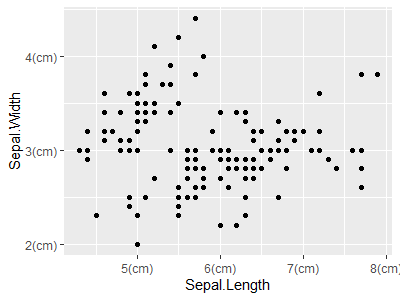
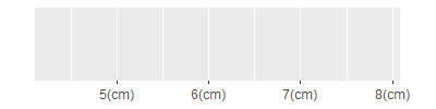
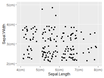
引数labels：軸の目盛りのラベル

labelsで軸の目盛りのラベルを指定できます。

R

ggplot(data = iris, aes(x = Sepal.Length, y = Sepal.Width)) +
  geom_point() +
  scale_x_continuous(breaks = 4:8,
                     labels = str_c(4:8, "(cm)")) +
  scale_y_continuous(breaks = 2:5,
                     labels = str_c(2:5, "(cm)"))

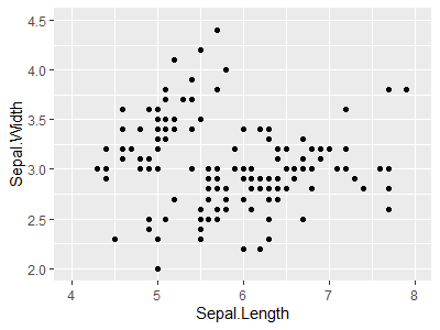
引数limits：軸の範囲

limitsで軸の範囲を指定できます。

R

ggplot(data = iris, aes(x = Sepal.Length, y = Sepal.Width)) +
  geom_point() +
  scale_x_continuous(limits = c(4, 8)) +
  scale_y_continuous(limits = c(2, 4.5))
ggplot(data = iris, aes(x = Sepal.Length, y = Sepal.Width)) +
  geom_point() +
  xlim(c(4, 8)) +
  ylim(c(2, 4.5))

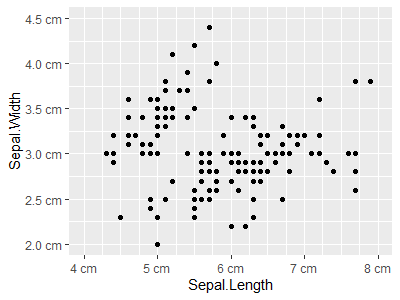
ここまでを全部合わせて

R

x_width <- 1.0
x_min <- floor(min(iris$Sepal.Length))    # 4
x_max <- ceiling(max(iris$Sepal.Length))  # 8
x_major_breaks <- seq(x_min, x_max, by = x_width)
x_major_breaks
# [1] 4 5 6 7 8
x_minor_breaks <- seq(x_min, x_max, by = x_width / 4)
x_minor_breaks
# [1] 4.00 4.25 4.50 4.75 5.00 5.25 5.50 5.75 6.00 6.25 6.50 6.75 7.00 7.25 7.50 7.75 8.00
y_width <- 0.5
y_min <- floor(min(iris$Sepal.Width) * 2) / 2   # 2
y_max <- ceiling(max(iris$Sepal.Width) * 2) / 2 # 4.5
y_major_breaks <- seq(y_min, y_max, by = y_width)
y_major_breaks
# [1] 2.0 2.5 3.0 3.5 4.0 4.5
y_minor_breaks <- seq(y_min, y_max, by = y_width / 2)
y_minor_breaks
# [1] 2.00 2.25 2.50 2.75 3.00 3.25 3.50 3.75 4.00 4.25 4.50
str_c(format(x_major_breaks, nsmall = 0), " cm")
sprintf("%d cm", x_major_breaks)
x_labels <- sprintf("%d cm", x_major_breaks)
x_labels
# [1] "4 cm" "5 cm" "6 cm" "7 cm" "8 cm"
str_c(format(y_major_breaks, nsmall = 1), " cm")
sprintf("%.1f cm", y_major_breaks)
y_labels <- sprintf("%.1f cm", y_major_breaks)
y_labels
# [1] "2.0 cm" "2.5 cm" "3.0 cm" "3.5 cm" "4.0 cm" "4.5 cm"
x_limits <- c(x_min, x_max)
x_limits
# [1] 4 8
y_limits <- c(y_min, y_max)
y_limits
# [1] 2.0 4.5
ggplot(data = iris, aes(x = Sepal.Length, y = Sepal.Width)) +
  geom_point() +
  scale_x_continuous(breaks = x_major_breaks, minor_breaks = x_minor_breaks,
                     labels = x_labels,
                     limits = x_limits) +
  scale_y_continuous(breaks = y_major_breaks, minor_breaks = y_minor_breaks,
                     labels = y_labels,
                     limits = y_limits)

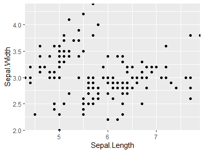
引数expand：値の範囲の外に拡張される軸の幅

expandで値の範囲の外に拡張される軸の幅を指定できます。

R

ggplot(data = iris, aes(x = Sepal.Length, y = Sepal.Width)) +
  geom_point() +
  scale_x_continuous(expand = c(0, 0)) +
  scale_y_continuous(expand = c(0, 0))
ggplot(data = iris, aes(x = Sepal.Length, y = Sepal.Width)) +
  geom_point() +
  scale_x_continuous(expand = expansion(mult = 0)) +
  scale_y_continuous(expand = expansion(mult = 0))
ggplot(data = iris, aes(x = Sepal.Length, y = Sepal.Width)) +
  geom_point() +
  scale_x_continuous(expand = expansion(add = 0)) +
  scale_y_continuous(expand = expansion(add = 0))

デフォルトでは、連続値の場合は値の範囲の5%外側までとなっています。

R

ggplot(data = iris, aes(x = Sepal.Length, y = Sepal.Width)) +
  geom_point() +
  scale_x_continuous() +
  scale_y_continuous()
ggplot(data = iris, aes(x = Sepal.Length, y = Sepal.Width)) +
  geom_point() +
  scale_x_continuous(expand = expansion(mult = 0.05)) + # デフォルト（値の範囲の5%）
  scale_y_continuous(expand = expansion(mult = 0.05))   # デフォルト（値の範囲の5%）
ggplot(data = iris, aes(x = Sepal.Length, y = Sepal.Width)) +
  geom_point() +
  scale_x_continuous(expand = expansion(add = diff(range(iris$Sepal.Length))*0.05)) +
  scale_y_continuous(expand = expansion(add = diff(range(iris$Sepal.Width))*0.05))

R

range(iris$Sepal.Length)
# [1] 4.3 7.9
diff(range(iris$Sepal.Length))
# [1] 3.6
diff(range(iris$Sepal.Length))*0.05
# [1] 0.18
min(iris$Sepal.Length) - diff(range(iris$Sepal.Length))*0.05
# [1] 4.12
max(iris$Sepal.Length) + diff(range(iris$Sepal.Length))*0.05
# [1] 8.08

range(iris$Sepal.Width)
# [1] 2.0 4.4
diff(range(iris$Sepal.Width))
# [1] 2.4
diff(range(iris$Sepal.Width))*0.05
# [1] 0.12
min(iris$Sepal.Width) - diff(range(iris$Sepal.Width))*0.05
# [1] 1.88
max(iris$Sepal.Width) + diff(range(iris$Sepal.Width))*0.05
# [1] 4.52

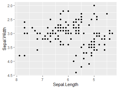
引数trans：軸のスケール変換

transで軸のスケール変換を行うことができます。
デフォルトでは"identity"で恒等変換です（何も変換されません。）。

R

ggplot(data = iris, aes(x = Sepal.Length, y = Sepal.Width)) +
  geom_point() +
  scale_x_continuous(trans = "identity") +  # デフォルト
  scale_y_continuous(trans = "identity")    # デフォルト

ggplot(data = iris, aes(x = Sepal.Length, y = Sepal.Width)) +
  geom_point() +
  scale_x_continuous(trans = "log10") +  # 常用対数変換
  scale_y_continuous(trans = "sqrt")     # sqrt変換
ggplot(data = iris, aes(x = Sepal.Length, y = Sepal.Width)) +
  geom_point() +
  scale_x_log10() +
  scale_y_sqrt()

ggplot(data = iris, aes(x = Sepal.Length, y = Sepal.Width)) +
  geom_point() +
  scale_x_continuous(trans = "reverse") +  # 軸の反転
  scale_y_continuous(trans = "reverse")    # 軸の反転
ggplot(data = iris, aes(x = Sepal.Length, y = Sepal.Width)) +
  geom_point() +
  scale_x_reverse() +
  scale_y_reverse()

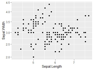
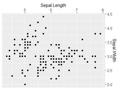
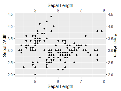
引数position：軸の表示場所

positionで軸を表示する場所を設定します。

R

ggplot(data = iris, aes(x = Sepal.Length, y = Sepal.Width)) +
  geom_point() +
  scale_x_continuous() +
  scale_y_continuous()
ggplot(data = iris, aes(x = Sepal.Length, y = Sepal.Width)) +
  geom_point() +
  scale_x_continuous(position = "bottom") +  # デフォルト
  scale_y_continuous(position = "left")      # デフォルト

ggplot(data = iris, aes(x = Sepal.Length, y = Sepal.Width)) +
  geom_point() +
  scale_x_continuous(position = "top") +
  scale_y_continuous(position = "right")

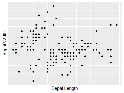
引数guide：軸の凡例

guideで軸の凡例を設定します。デフォルトでは通常の軸が表示されます。
また、これはguides()でも設定できます。scale_x_continuous(guide = ...)とguides(x = ...)は同じです。

R

ggplot(data = iris, aes(x = Sepal.Length, y = Sepal.Width)) +
  geom_point() +
  scale_x_continuous(guide = guide_axis()) +  # デフォルト
  scale_y_continuous(guide = guide_axis())    # デフォルト
ggplot(data = iris, aes(x = Sepal.Length, y = Sepal.Width)) +
  geom_point() +
  scale_x_continuous(guide = "axis") +  # デフォルト
  scale_y_continuous(guide = "axis")    # デフォルト
ggplot(data = iris, aes(x = Sepal.Length, y = Sepal.Width)) +
  geom_point() +
  guides(x = guide_axis()) +  # デフォルト
  guides(y = guide_axis())    # デフォルト
ggplot(data = iris, aes(x = Sepal.Length, y = Sepal.Width)) +
  geom_point() +
  guides(x = "axis") +  # デフォルト
  guides(y = "axis")    # デフォルト

guideにNULLか"none"を指定すると、軸が表示されなくなります。

R

ggplot(data = iris, aes(x = Sepal.Length, y = Sepal.Width)) +
  geom_point() +
  scale_x_continuous(guide = NULL) +
  scale_y_continuous(guide = NULL)
ggplot(data = iris, aes(x = Sepal.Length, y = Sepal.Width)) +
  geom_point() +
  scale_x_continuous(guide = "none") +
  scale_y_continuous(guide = "none")
ggplot(data = iris, aes(x = Sepal.Length, y = Sepal.Width)) +
  geom_point() +
  guides(x = "none") +
  guides(y = "none")

さらに、guide_axis()関数で詳細を設定できます。

guide_axis()：軸の凡例を設定する関数

scale_x_continuous(guide = guide_axis(... ))とguides(x = guide_axis(... ))は同じです。

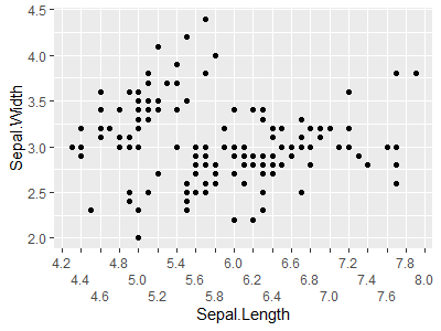
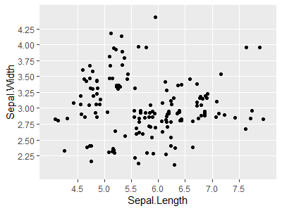
引数n.dodge：軸のラベルを複数列にずらして表示

通常、軸のラベルは一列に表示されますが、重なったり近すぎたりして見づらい場合などずらして表示したいときがあります。n.dodgeで複数列にずらして表示できます。

R

ggplot(data = iris, aes(x = Sepal.Length, y = Sepal.Width)) +
  geom_point() +
  scale_x_continuous(breaks = seq(4, 8, by = 0.2), minor_breaks = NULL)
ggplot(data = iris, aes(x = Sepal.Length, y = Sepal.Width)) +
  geom_point() +
  scale_x_continuous(breaks = seq(4, 8, by = 0.2), minor_breaks = NULL,
                     guide = guide_axis(n.dodge = 1))  # デフォルト
ggplot(data = iris, aes(x = Sepal.Length, y = Sepal.Width)) +
  geom_point() +
  scale_x_continuous(breaks = seq(4, 8, by = 0.2), minor_breaks = NULL) +
  guides(x = guide_axis(n.dodge = 1))  # デフォルト

ggplot(data = iris, aes(x = Sepal.Length, y = Sepal.Width)) +
  geom_point() +
  scale_x_continuous(breaks = seq(4, 8, by = 0.2), minor_breaks = NULL,
                     guide = guide_axis(n.dodge = 2))
ggplot(data = iris, aes(x = Sepal.Length, y = Sepal.Width)) +
  geom_point() +
  scale_x_continuous(breaks = seq(4, 8, by = 0.2), minor_breaks = NULL) +
  guides(x = guide_axis(n.dodge = 2))

ggplot(data = iris, aes(x = Sepal.Length, y = Sepal.Width)) +
  geom_point() +
  scale_x_continuous(breaks = seq(4, 8, by = 0.2), minor_breaks = NULL,
                     guide = guide_axis(n.dodge = 3))
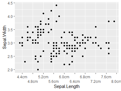
ggplot(data = iris, aes(x = Sepal.Length, y = Sepal.Width)) +
  geom_point() +
  scale_x_continuous(breaks = seq(4, 8, by = 0.4), minor_breaks = NULL,
                     labels = sprintf("%.1fcm", seq(4, 8, by = 0.4))) +
  guides(x = guide_axis(n.dodge = 2))

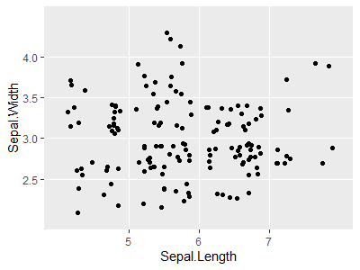
引数angle：軸のラベルの表示の角度

angleで軸のラベルの表示の角度を指定できます。

R

ggplot(data = iris, aes(x = Sepal.Length, y = Sepal.Width)) +
  geom_point() +
  scale_x_continuous(breaks = seq(4, 8, by = 0.2), minor_breaks = NULL,
                     labels = sprintf("%.1f cm", seq(4, 8, by = 0.2)),
                     guide = guide_axis(angle = 90))
ggplot(data = iris, aes(x = Sepal.Length, y = Sepal.Width)) +
  geom_point() +
  scale_x_continuous(breaks = seq(4, 8, by = 0.2), minor_breaks = NULL,
                     labels = sprintf("%.1f cm", seq(4, 8, by = 0.2))) +
  guides(x = guide_axis(angle = 90))

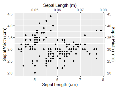
引数sec.axis：第２軸

sec.axisで第２軸の設定ができます。
sec.axisにdup_axis()を指定すると、第１軸と同じ軸が複製されます。
新たな第２軸を作成するには、sec_axis()関数を使えます。

R

ggplot(data = iris, aes(x = Sepal.Length, y = Sepal.Width)) +
  geom_point() +
  scale_x_continuous(sec.axis = dup_axis()) +  # 軸の複製
  scale_y_continuous(sec.axis = dup_axis())    # 軸の複製
ggplot(data = iris, aes(x = Sepal.Length, y = Sepal.Width)) +
  geom_point() +
  scale_x_continuous(sec.axis = sec_axis(trans = ~ ., name = derive())) +
  scale_y_continuous(sec.axis = sec_axis(trans = ~ ., name = derive()))
ggplot(data = iris, aes(x = Sepal.Length, y = Sepal.Width)) +
  geom_point() +
  guides(x.sec = guide_axis(title = "Sepal.Length"),
         y.sec = guide_axis(title = "Sepal.Width"))

ggplot(data = iris, aes(x = Sepal.Length, y = Sepal.Width)) +
  geom_point() +
  scale_x_continuous(name = "Sepal Length (cm)",
                     sec.axis = sec_axis(trans = ~ . / 100, name = "Sepal Length (m)")) +
  scale_y_continuous(name = "Sepal Width (cm)",
                     sec.axis = sec_axis(trans = ~ . * 10,  name = "Sepal Width (mm)"))

R

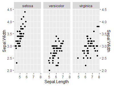
ggplot(data = iris, aes(x = Sepal.Length, y = Sepal.Width)) +
  geom_point() +
  facet_grid(cols = vars(Species)) +
  scale_y_continuous(sec.axis = dup_axis())

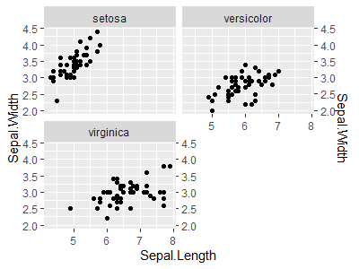
ggplot(data = iris, aes(x = Sepal.Length, y = Sepal.Width)) +
  geom_point() +
  facet_wrap(facets = vars(Species), ncol = 2) +
  scale_y_continuous(sec.axis = dup_axis())

（注）scalesライブラリのdemo_continuous()関数で連続値の軸のスケーリングのデモンストレーションを見ることもできます。

R

library(scales)
demo_continuous(iris$Sepal.Length)

demo_continuous(iris$Sepal.Length, breaks = seq(4, 8, by = 0.5))

demo_continuous(iris$Sepal.Length, breaks = 4:8, minor_breaks = seq(4, 8, by = 0.2))

demo_continuous(iris$Sepal.Length, breaks = 4:8, minor_breaks = NULL)

demo_continuous(iris$Sepal.Length, breaks = 4:8, labels = str_c(4:8, "(cm)"))

demo_continuous(iris$Sepal.Length, breaks = 4:8, limits = c(4, 8))

demo_continuous(iris$Sepal.Length, breaks = 4:8, expand = c(0, 0))

demo_continuous(iris$Sepal.Length, breaks = 4:8, trans = "reverse")

scale_x_discrete(), scale_y_discrete()：離散値のx軸, y軸

x軸, y軸が離散値の場合、scale_x_discrete(), scale_y_discrete()で軸の設定を調整します。

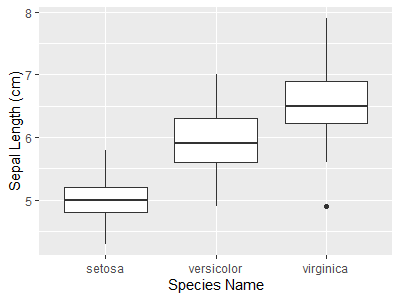
引数name：軸のラベル

scale_x_continuous(), scale_x_continuous()と同じく、scale_x_discrete(), scale_y_discrete()でもnameで軸のラベルに表示される文字列を設定できます。
xlab(), ylab()でも設定できます。

R

ggplot(data = iris, aes(x = Species, y = Sepal.Length)) +
  geom_boxplot() +
  scale_x_discrete(name = "Species Name") +
  scale_y_continuous(name = "Sepal Length (cm)")
ggplot(data = iris, aes(x = Species, y = Sepal.Length)) +
  geom_boxplot() +
  xlab("Species Name") +
  ylab("Sepal Length (cm)")

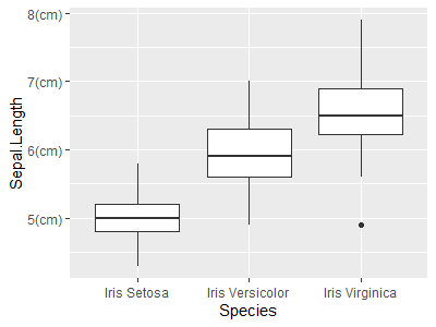
引数labels：軸の目盛りのラベル

scale_x_continuous(), scale_x_continuous()と同じく、scale_x_discrete(), scale_y_discrete()でもlabelsで軸の目盛りのラベルを指定できます。

R

ggplot(data = iris, aes(x = Species, y = Sepal.Length)) +
  geom_boxplot() +
  scale_x_discrete(labels = str_c("Iris ", str_to_title(unique(iris$Species)))) +
  scale_y_continuous(labels = str_c(4:8, "(cm)"))

unique(iris$Species)
# [1] setosa     versicolor virginica 
# Levels: setosa versicolor virginica
str_c("Iris ", str_to_title(unique(iris$Species)))
# [1] "Iris Setosa"     "Iris Versicolor" "Iris Virginica" 

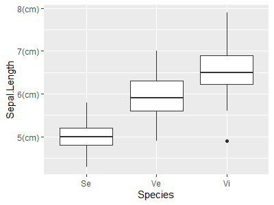
ggplot(data = iris, aes(x = Species, y = Sepal.Length)) +
  geom_boxplot() +
  scale_x_discrete(labels = c("setosa" = "Se", "versicolor" = "Ve", "virginica"  = "Vi")) +
  scale_y_continuous(labels = str_c(4:8, "(cm)"))

c("setosa" = "Se", "versicolor" = "Ve", "virginica"  = "Vi")
#     setosa versicolor  virginica 
#       "Se"       "Ve"       "Vi" 

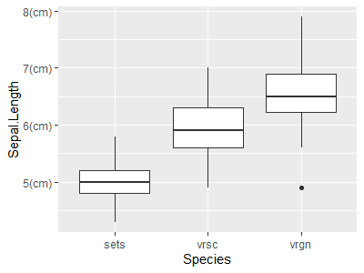
ggplot(data = iris, aes(x = Species, y = Sepal.Length)) +
  geom_boxplot() +
  scale_x_discrete(labels = abbreviate) +
  scale_y_continuous(labels = str_c(4:8, "(cm)"))

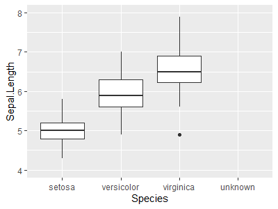
引数limits：軸の範囲

scale_x_continuous(), scale_x_continuous()と同じく、scale_x_discrete(), scale_y_discrete()でもlimitsで軸の範囲を指定できます（表示するすべての値をベクトルで与えます。順序も反映されます。）。

R

ggplot(data = iris, aes(x = Species, y = Sepal.Length)) +
  geom_boxplot() +
  scale_x_discrete(limits = c("setosa", "versicolor", "virginica", "unknown")) +
  scale_y_continuous(limits = c(4, 8))

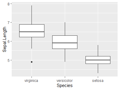
これを用いると軸の反転もできます。連続値の場合と違って、trans = "reverse"で反転することはできません。

R

ggplot(data = iris, aes(x = Species, y = Sepal.Length)) +
  geom_boxplot() +
  scale_x_discrete(limits = c("virginica", "versicolor", "setosa"))
ggplot(data = iris, aes(x = Species, y = Sepal.Length)) +
  geom_boxplot() +
  scale_x_discrete(limits = rev(unique(iris$Species)))
rev(unique(iris$Species))
# [1] virginica  versicolor setosa    
# Levels: setosa versicolor virginica

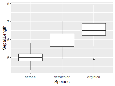
引数expand：値の範囲の外に拡張される軸の幅

scale_x_continuous(), scale_x_continuous()と同じく、scale_x_discrete(), scale_y_discrete()でもexpandで値の範囲の外に拡張される軸の幅を指定できます。
離散値の場合、デフォルトは単位の0.6倍外側となっています。

R

ggplot(data = iris, aes(x = Species, y = Sepal.Length)) +
  geom_boxplot() +
  scale_x_discrete() +
  scale_y_continuous()
ggplot(data = iris, aes(x = Species, y = Sepal.Length)) +
  geom_boxplot() +
  scale_x_discrete(expand = expansion(add = 0.6)) +    # デフォルト（単位の0.6倍）
  scale_y_continuous(expand = expansion(mult = 0.05))  # デフォルト（値の範囲の5%）

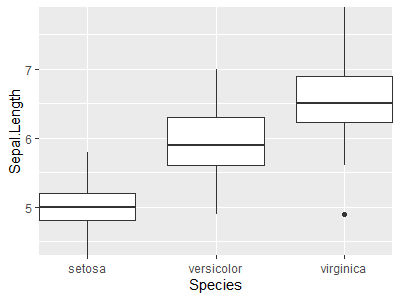
ggplot(data = iris, aes(x = Species, y = Sepal.Length)) +
  geom_boxplot() +
  scale_x_discrete(expand = expansion(add = 0)) +
  scale_y_continuous(expand = expansion(add = 0))

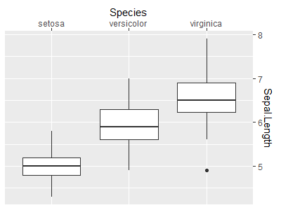
引数position：軸の表示場所

scale_x_continuous(), scale_x_continuous()と同じく、scale_x_discrete(), scale_y_discrete()でもpositionで軸の表示場所をを指定できます。

R

ggplot(data = iris, aes(x = Species, y = Sepal.Length)) +
  geom_boxplot() +
  scale_x_discrete() +
  scale_y_continuous()
ggplot(data = iris, aes(x = Species, y = Sepal.Length)) +
  geom_boxplot() +
  scale_x_discrete(position = "bottom") +  # デフォルト
  scale_y_continuous(position = "left")    # デフォルト

ggplot(data = iris, aes(x = Species, y = Sepal.Length)) +
  geom_boxplot() +
  scale_x_discrete(position = "top") +
  scale_y_continuous(position = "right")

引数guide：軸の凡例

scale_x_continuous(), scale_x_continuous()と同じく、scale_x_discrete(), scale_y_discrete()でもguideで軸の凡例を設定します。デフォルトでは通常の軸が表示されます。

R

ggplot(data = iris, aes(x = Species, y = Sepal.Length)) +
  geom_boxplot() +
  scale_x_discrete(guide = guide_axis()) +  # デフォルト
  scale_y_continuous(guide = guide_axis())  # デフォルト
ggplot(data = iris, aes(x = Species, y = Sepal.Length)) +
  geom_boxplot() +
  scale_x_discrete(guide = "axis") +  # デフォルト
  scale_y_continuous(guide = "axis")  # デフォルト
ggplot(data = iris, aes(x = Species, y = Sepal.Length)) +
  geom_boxplot() +
  guides(x = guide_axis()) +  # デフォルト
  guides(y = guide_axis())    # デフォルト
ggplot(data = iris, aes(x = Species, y = Sepal.Length)) +
  geom_boxplot() +
  guides(x = "axis") +  # デフォルト
  guides(y = "axis")    # デフォルト

guide_axis()：軸の凡例を設定する関数

scale_x_discrete(guide = guide_axis(... ))とguides(x = guide_axis(... ))は同じです。

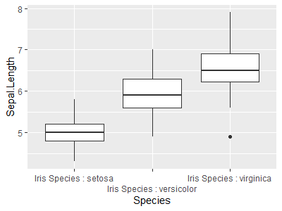
引数n.dodge：軸のラベルを複数列にずらして表示

scale_x_continuous(), scale_x_continuous()と同じく、scale_x_discrete(), scale_y_discrete()の中でもguide_axis()関数の引数n.dodgeで複数列にずらして表示できます。

R

ggplot(data = iris, aes(x = Species, y = Sepal.Length)) +
  geom_boxplot() +
  scale_x_discrete(guide = guide_axis(n.dodge = 1)) +  # デフォルト
  scale_y_continuous(guide = guide_axis(n.dodge = 1))  # デフォルト
ggplot(data = iris, aes(x = Species, y = Sepal.Length)) +
  geom_boxplot() +
  guides(x = guide_axis(n.dodge = 1)) +  # デフォルト
  guides(y = guide_axis(n.dodge = 1))    # デフォルト

ggplot(data = iris, aes(x = Species, y = Sepal.Length)) +
  geom_boxplot() +
  scale_x_discrete(labels = str_c("Iris Species : ", unique(iris$Species)),
                   guide = guide_axis(n.dodge = 2))

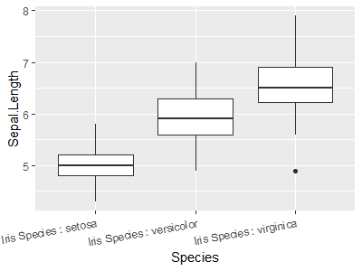
引数angle：軸のラベルの表示の角度

scale_x_continuous(), scale_x_continuous()と同じく、scale_x_discrete(), scale_y_discrete()の中でもguide_axis()関数の引数angleで軸のラベルの表示の角度を指定できます。

R

ggplot(data = iris, aes(x = Species, y = Sepal.Length)) +
  geom_boxplot() +
  scale_x_discrete(labels = str_c("Iris Species : ", unique(iris$Species)),
                   guide = guide_axis(angle = 10))

scale_x_binned(), scale_y_binned()：連続値のx軸, y軸のビン分割

x軸, y軸が連続値の場合、連続値をビンで区分します。

R

ggplot(data = iris, aes(x = Sepal.Length, y = Sepal.Width)) +
  geom_jitter() +
  scale_x_binned() +
  scale_y_binned()

R

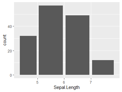
ggplot(data = iris, aes(x = Sepal.Length)) +
  geom_bar(width = 0.9) +
  scale_x_binned()

引数name：軸のラベル

R

ggplot(data = iris, aes(x = Sepal.Length, y = Sepal.Width)) +
  geom_jitter() +
  scale_x_binned(name = "Sepal Length (cm)") +
  scale_y_binned(name = "Sepal Width (cm)")

ggplot(data = iris, aes(x = Sepal.Length)) +
  geom_bar(width = 0.9) +
  scale_x_binned(name = "Sepal Length (cm)")

引数n.breaks, nice.breaks

R

ggplot(data = iris, aes(x = Sepal.Length, y = Sepal.Width)) +
  geom_jitter() +
  scale_x_binned(n.breaks = 4) +
  scale_y_binned(n.breaks = 5)
ggplot(data = iris, aes(x = Sepal.Length, y = Sepal.Width)) +
  geom_jitter() +
  scale_x_binned(n.breaks = 4, nice.breaks = TRUE) +
  scale_y_binned(n.breaks = 5, nice.breaks = TRUE)

ggplot(data = iris, aes(x = Sepal.Length, y = Sepal.Width)) +
  geom_jitter() +
  scale_x_binned(n.breaks = 4, nice.breaks = FALSE) +
  scale_y_binned(n.breaks = 5, nice.breaks = FALSE)

R

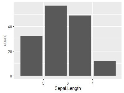
ggplot(data = iris, aes(x = Sepal.Length)) +
  geom_bar(width = 0.9) +
  scale_x_binned(n.breaks = 4)
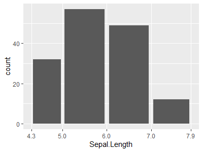
ggplot(data = iris, aes(x = Sepal.Length)) +
  geom_bar(width = 0.9) +
  scale_x_binned(n.breaks = 4, nice.breaks = TRUE)

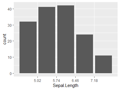
ggplot(data = iris, aes(x = Sepal.Length)) +
  geom_bar(width = 0.9) +
  scale_x_binned(n.breaks = 4, nice.breaks = FALSE)

引数show.limits

R

ggplot(data = iris, aes(x = Sepal.Length)) +
  geom_bar(width = 0.9) +
  scale_x_binned(breaks = 4:8)
ggplot(data = iris, aes(x = Sepal.Length)) +
  geom_bar(width = 0.9) +
  scale_x_binned(breaks = 4:8,
                 show.limits = FALSE)

ggplot(data = iris, aes(x = Sepal.Length)) +
  geom_bar(width = 0.9) +
  scale_x_binned(breaks = 4:8,
                 show.limits = TRUE)

引数breaks：軸の目盛り

R

ggplot(data = iris, aes(x = Sepal.Length)) +
  geom_bar(width = 0.9) +
  scale_x_binned(breaks = 4:8)
ggplot(data = iris, aes(x = Sepal.Length)) +
  geom_bar(width = 0.9) +
  scale_x_binned(breaks = 4:8,
                 show.limits = FALSE)

ggplot(data = iris, aes(x = Sepal.Length)) +
  geom_bar(width = 0.9) +
  scale_x_binned(breaks = 4:8,
                 show.limits = TRUE)

R

ggplot(data = iris, aes(x = Sepal.Length, y = Sepal.Width)) +
  geom_jitter() +
  scale_x_binned(breaks = 4:8,
                 show.limits = TRUE) +
  scale_y_binned(breaks = 2:5,
                 show.limits = TRUE)

引数limits：軸の範囲

R

ggplot(data = iris, aes(x = Sepal.Length, y = Sepal.Width)) +
  geom_jitter() +
  scale_x_binned(limits = c(4, 8)) +
  scale_y_binned(limits = c(2, 5))

引数labels：軸の目盛りのラベル

R

ggplot(data = iris, aes(x = Sepal.Length, y = Sepal.Width)) +
  geom_jitter() +
  scale_x_binned(breaks = 4:8,
                 limits = c(4, 8),
                 labels = str_c(4:8, "(cm)")) +
  scale_y_binned(breaks = 2:5,
                 limits = c(2, 5),
                 labels = str_c(2:5, "(cm)"))

引数trans：軸のスケール変換

R

ggplot(data = iris, aes(x = Sepal.Length, y = Sepal.Width)) +
  geom_jitter() +
  scale_x_binned(trans = "log10") +
  scale_y_binned(trans = "sqrt")

scale_color_*(), scale_fill_*(), scale_alpha_*(), scale_size_*(), scale_shape_*(), scale_linetype_*()：color軸, fill軸, alpha軸, shape軸, size軸, linetype軸

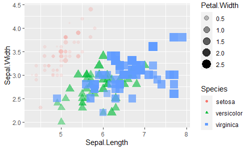
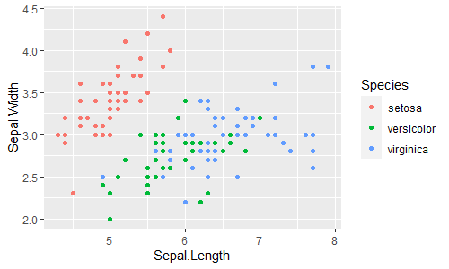
ggplot2では、x軸・y軸の2次元以外に、color¹軸, fill軸などもaes()に指定することで設定できます。
これらの軸は、デフォルトでは、連続値のcolor軸はカラーバー表示、それ以外は通常の凡例表示になります。

R

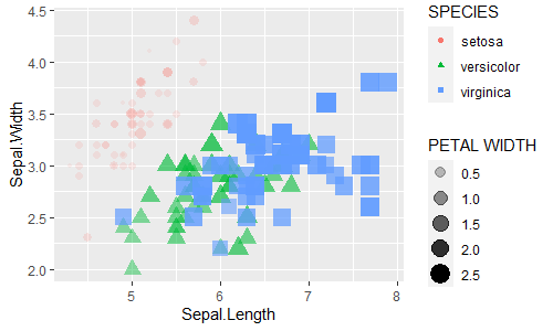
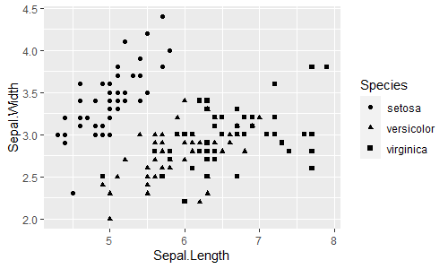
ggplot(data = iris, aes(x = Sepal.Length, y = Sepal.Width)) +
  geom_point(aes(shape = Species,
                 color = Species,
                 size  = Petal.Width,
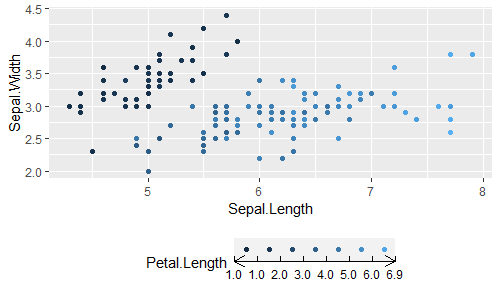
                 alpha = Petal.Width))

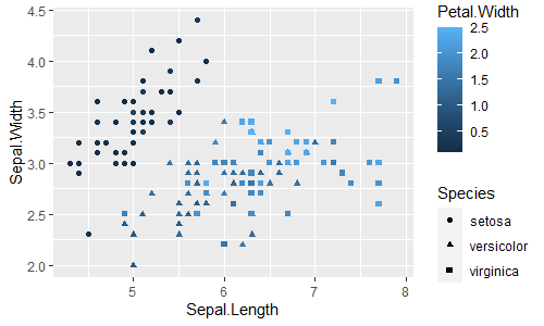
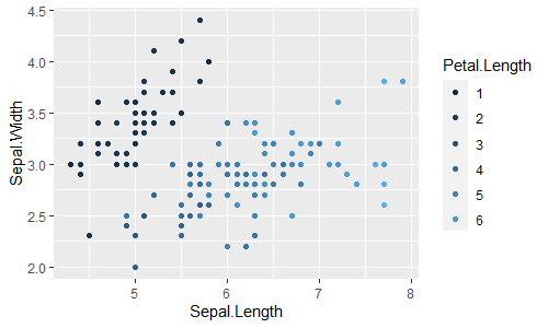
ggplot(data = iris, aes(x = Sepal.Length, y = Sepal.Width)) +
  geom_point(aes(shape = Species,
                 color = Petal.Width))

scale_*_continuous()：連続値のcolor軸など

scale_*_discrete()：離散値のcolor軸など

scale_*_binned()：連続値のcolor軸などのビン分割

x軸・y軸と同様に、color軸などの設定も、連続値か離散値かによってscale_*_continuous(), scale_*_discrete()（連続値をビン分割する場合はscale_*_binned()）を使います。

• scale_*_continuous()：連続（continuous）値の場合
• scale_*_discrete()：離散（discrete）値の場合
• scale_*_binned()：連続（continuous）値の場合（ビン分割）

引数name：軸のラベル

scale_x_continuous(), scale_x_discrete(), scale_x_binned()などと同様です。labs()でも設定できます。

R

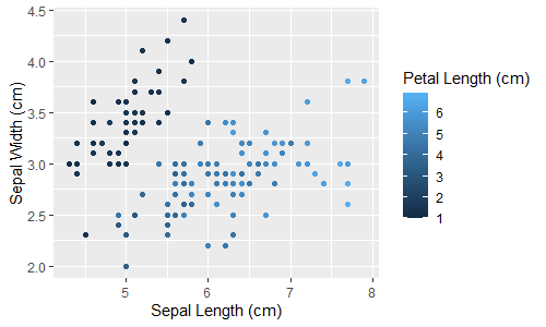
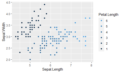
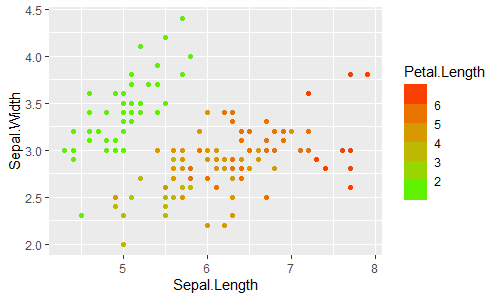
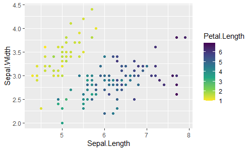
ggplot(data = iris, aes(x = Sepal.Length, y = Sepal.Width)) +
  geom_point(aes(color = Petal.Length)) +
  scale_x_continuous(name = "Sepal Length (cm)") +
  scale_y_continuous(name = "Sepal Width (cm)") +
  scale_color_continuous(name = "Petal Length (cm)")
ggplot(data = iris, aes(x = Sepal.Length, y = Sepal.Width)) +
  geom_point(aes(color = Petal.Length)) +
  labs(x = "Sepal Length (cm)",
       y = "Sepal Width (cm)",
       color = "Petal Length (cm)")

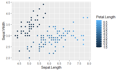
ggplot(data = iris, aes(x = Sepal.Length, y = Sepal.Width)) +
  geom_point(aes(color = Petal.Length)) +
  scale_x_continuous(name = "Sepal Length (cm)") +
  scale_y_continuous(name = "Sepal Width (cm)") +
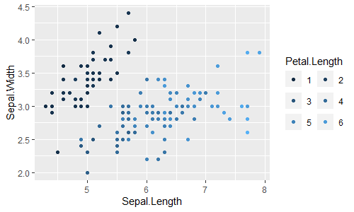
  scale_color_binned(name = "Petal Length (cm)")

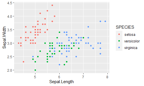
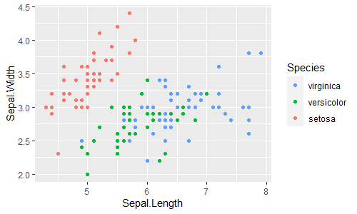
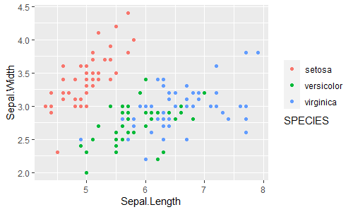
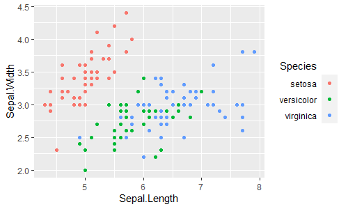
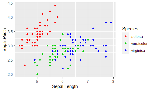
ggplot(data = iris, aes(x = Sepal.Length, y = Sepal.Width)) +
  geom_point(aes(color = Species)) +
  scale_color_discrete(name = "SPECIES")
ggplot(data = iris, aes(x = Sepal.Length, y = Sepal.Width)) +
  geom_point(aes(color = Species)) +
  labs(color = "SPECIES")

引数breaks：軸の目盛り

軸の変数が連続値の場合、scale_x_continuous()と同様に軸の目盛りを設定できます。

R

ggplot(data = iris, aes(x = Sepal.Length, y = Sepal.Width)) +
  geom_point(aes(color = Petal.Length)) +
  scale_x_continuous(breaks = seq(4, 8, by = 0.5)) +
  scale_y_continuous(breaks = seq(2, 5, by = 0.5)) +
  scale_color_continuous(breaks = seq(0, 7, by = 0.5))

R

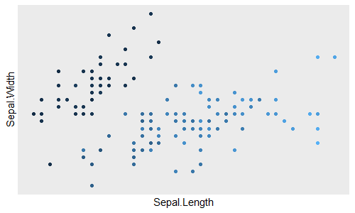
ggplot(data = iris, aes(x = Sepal.Length, y = Sepal.Width)) +
  geom_point(aes(color = Petal.Length)) +
  scale_x_continuous(breaks = NULL) +
  scale_y_continuous(breaks = NULL) +
  scale_color_continuous(breaks = NULL)

また、breaksは等間隔でなくてもかまいません。

R

ggplot(data = iris, aes(x = Sepal.Length, y = Sepal.Width)) +
  geom_point(aes(color = Petal.Length)) +
  scale_color_continuous(breaks = c(1, 2, 4, 8))

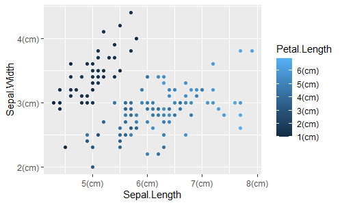
引数labels：軸の目盛りのラベル

R

ggplot(data = iris, aes(x = Sepal.Length, y = Sepal.Width)) +
  geom_point(aes(color = Petal.Length)) +
  scale_x_continuous(breaks = 4:8,
                     labels = str_c(4:8, "(cm)")) +
  scale_y_continuous(breaks = 2:5,
                     labels = str_c(2:5, "(cm)")) +
  scale_color_continuous(breaks = 1:7,
                         labels = str_c(1:7, "(cm)"))

引数limits：軸の範囲

R

ggplot(data = iris, aes(x = Sepal.Length, y = Sepal.Width)) +
  geom_point(aes(color = Petal.Length)) +
  scale_x_continuous(limits = c(4, 8)) +
  scale_y_continuous(limits = c(2, 4.5)) +
  scale_color_continuous(limits = c(1, 7))

引数trans：軸のスケール変換

R

ggplot(data = iris, aes(x = Sepal.Length, y = Sepal.Width)) +
  geom_point(aes(color = Petal.Length)) +
  scale_color_continuous(trans = "sqrt")

ggplot(data = iris, aes(x = Sepal.Length, y = Sepal.Width)) +
  geom_point(aes(color = Petal.Length)) +
  scale_color_continuous(trans = "reverse")

引数guide：軸の凡例

凡例の表示の設定です。
デフォルトでは、連続値のcolor軸はカラーバー表示guide = "colorbar"、それ以外は通常の凡例表示guide = "legend"です。
scale_*_discrete(guide = ...), scale_*_continuous()とguides(* = ...)は同じです。また、guides()の中身はまとめても書けます。

R

ggplot(data = iris, aes(x = Sepal.Length, y = Sepal.Width)) +
  geom_point(aes(shape = Species,
                 color = Species,
                 size  = Petal.Width,
                 alpha = Petal.Width)) +
  scale_shape_discrete(guide = "legend") +  # デフォルト
  scale_color_discrete(guide = "legend") +  # デフォルト
  scale_size_continuous(guide = "legend") + # デフォルト
  scale_alpha_continuous(guide = "legend")  # デフォルト
ggplot(data = iris, aes(x = Sepal.Length, y = Sepal.Width)) +
  geom_point(aes(shape = Species,
                 color = Species,
                 size  = Petal.Width,
                 alpha = Petal.Width)) +
  guides(shape = "legend") +  # デフォルト
  guides(color = "legend") +  # デフォルト
  guides(size  = "legend") +  # デフォルト
  guides(alpha = "legend")    # デフォルト
ggplot(data = iris, aes(x = Sepal.Length, y = Sepal.Width)) +
  geom_point(aes(shape = Species,
                 color = Species,
                 size  = Petal.Width,
                 alpha = Petal.Width)) +
  guides(shape = "legend",  # デフォルト
         color = "legend",  # デフォルト
         size  = "legend",  # デフォルト
         alpha = "legend")  # デフォルト

ggplot(data = iris, aes(x = Sepal.Length, y = Sepal.Width)) +
  geom_point(aes(shape = Species,
                 color = Petal.Width)) +
  scale_shape_discrete(guide = "legend") +   # デフォルト
  scale_color_continuous(guide = "colorbar") # デフォルト
ggplot(data = iris, aes(x = Sepal.Length, y = Sepal.Width)) +
  geom_point(aes(shape = Species,
                 color = Petal.Width)) +
  guides(shape = "legend") + # デフォルト
  guides(color = "colorbar") # デフォルト
ggplot(data = iris, aes(x = Sepal.Length, y = Sepal.Width)) +
  geom_point(aes(shape = Species,
                 color = Petal.Width)) +
  guides(shape = "legend",   # デフォルト
         color = "colorbar") # デフォルト

連続値のcolor軸も通常の通常の凡例表示guide = "legend"にできます。

R

ggplot(data = iris, aes(x = Sepal.Length, y = Sepal.Width)) +
  geom_point(aes(color = Petal.Length)) +
  scale_color_continuous(guide = "legend")
ggplot(data = iris, aes(x = Sepal.Length, y = Sepal.Width)) +
  geom_point(aes(color = Petal.Length)) +
  guides(color = "legend")

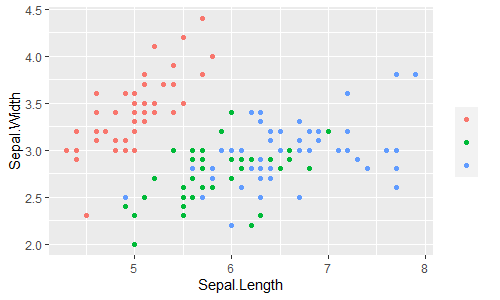
guide = "none"かguide = FALSEとすれば、凡例が表示されなくなります。

R

ggplot(data = iris, aes(x = Sepal.Length, y = Sepal.Width)) +
  geom_point(aes(shape = Species,
                 color = Species,
                 size  = Petal.Width,
                 alpha = Petal.Width)) +
  scale_shape_discrete(guide = "none") +
  scale_color_discrete(guide = "none") +
  scale_size_continuous(guide = NULL) +
  scale_alpha_continuous(guide = NULL)
ggplot(data = iris, aes(x = Sepal.Length, y = Sepal.Width)) +
  geom_point(aes(shape = Species,
                 color = Species,
                 size  = Petal.Width,
                 alpha = Petal.Width)) +
  guides(shape = "none") +
  guides(color = "none") +
  guides(size  = "none") +
  guides(alpha = "none")
ggplot(data = iris, aes(x = Sepal.Length, y = Sepal.Width)) +
  geom_point(aes(shape = Species,
                 color = Species,
                 size  = Petal.Width,
                 alpha = Petal.Width)) +
  guides(shape = "none",
         color = "none",
         size  = "none",
         alpha = "none")

R

ggplot(data = iris, aes(x = Sepal.Length, y = Sepal.Width)) +
  geom_point(aes(shape = Species,
                 color = Species,
                 size  = Petal.Width,
                 alpha = Petal.Width)) +
  guides(shape = "legend",
         color = "legend",
         size  = "none",
         alpha = "none")
ggplot(data = iris, aes(x = Sepal.Length, y = Sepal.Width)) +
  geom_point(aes(shape = Species,
                 color = Species,
                 size  = Petal.Width,
                 alpha = Petal.Width)) +
  guides(size  = "none",
         alpha = "none")

さらに、guide_legend()関数, guide_colorbar()関数で詳細を設定できます。

guide_legend()：凡例を設定する関数

scale_***_discrete(guide = guide_legend(... ))とguides(*** = guide_legend(... ))は同じです。
scale_***_continuous(guide = guide_legend(... ))とguides(*** = guide_legend(... ))は同じです。

R

ggplot(data = iris, aes(x = Sepal.Length, y = Sepal.Width)) +
  geom_point(aes(color = Species))
ggplot(data = iris, aes(x = Sepal.Length, y = Sepal.Width)) +
  geom_point(aes(color = Species)) +
  scale_color_discrete()
ggplot(data = iris, aes(x = Sepal.Length, y = Sepal.Width)) +
  geom_point(aes(color = Species)) +
  scale_color_discrete(guide = "legend")
ggplot(data = iris, aes(x = Sepal.Length, y = Sepal.Width)) +
  geom_point(aes(color = Species)) +
  scale_color_discrete(guide = guide_legend())
ggplot(data = iris, aes(x = Sepal.Length, y = Sepal.Width)) +
  geom_point(aes(color = Species)) +
  guides(color = "legend")
ggplot(data = iris, aes(x = Sepal.Length, y = Sepal.Width)) +
  geom_point(aes(color = Species)) +
  guides(color = guide_legend())

R

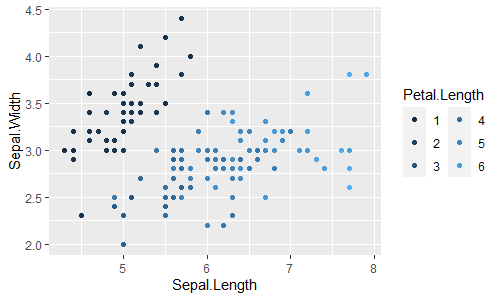
ggplot(data = iris, aes(x = Sepal.Length, y = Sepal.Width)) +
  geom_point(aes(color = Petal.Length)) +
  scale_color_continuous(guide = "legend")
ggplot(data = iris, aes(x = Sepal.Length, y = Sepal.Width)) +
  geom_point(aes(color = Petal.Length)) +
  scale_color_continuous(guide = guide_legend())
ggplot(data = iris, aes(x = Sepal.Length, y = Sepal.Width)) +
  geom_point(aes(color = Petal.Length)) +
  guides(color = "legend")
ggplot(data = iris, aes(x = Sepal.Length, y = Sepal.Width)) +
  geom_point(aes(color = Petal.Length)) +
  guides(color = guide_legend())

R

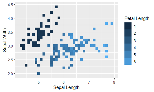
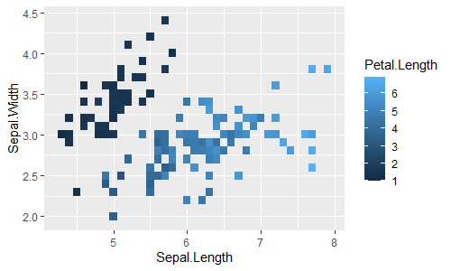
ggplot(data = iris, aes(x = Sepal.Length, y = Sepal.Width)) +
  geom_tile(aes(fill = Petal.Length)) +
  guides(fill = "legend")
ggplot(data = iris, aes(x = Sepal.Length, y = Sepal.Width)) +
  geom_tile(aes(fill = Petal.Length)) +
  guides(fill = guide_legend())

R

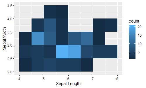
ggplot(data = iris, aes(x = Sepal.Length, y = Sepal.Width)) +
  geom_bin2d(stat = "bin2d", binwidth = 0.5) +
  scale_fill_continuous(guide = "legend")
ggplot(data = iris, aes(x = Sepal.Length, y = Sepal.Width)) +
  geom_bin2d(stat = "bin2d", binwidth = 0.5) +
  scale_fill_continuous(guide = guide_legend())
ggplot(data = iris, aes(x = Sepal.Length, y = Sepal.Width)) +
  geom_bin2d(stat = "bin2d", binwidth = 0.5) +
  guides(fill = "legend")
ggplot(data = iris, aes(x = Sepal.Length, y = Sepal.Width)) +
  geom_bin2d(stat = "bin2d", binwidth = 0.5) +
  guides(fill = guide_legend())

引数reverse：凡例の軸の反転

凡例の軸の表示を反転させます。

R

ggplot(data = iris, aes(x = Sepal.Length, y = Sepal.Width)) +
  geom_point(aes(color = Species)) +
  guides(color = guide_legend())
ggplot(data = iris, aes(x = Sepal.Length, y = Sepal.Width)) +
  geom_point(aes(color = Species)) +
  guides(color = guide_legend(reverse = FALSE))  # デフォルト

ggplot(data = iris, aes(x = Sepal.Length, y = Sepal.Width)) +
  geom_point(aes(color = Species)) +
  guides(color = guide_legend(reverse = TRUE))

R

ggplot(data = iris, aes(x = Sepal.Length, y = Sepal.Width)) +
  geom_point(aes(color = Petal.Length)) +
  guides(color = guide_legend())
ggplot(data = iris, aes(x = Sepal.Length, y = Sepal.Width)) +
  geom_point(aes(color = Petal.Length)) +
  guides(color = guide_legend(reverse = FALSE))

ggplot(data = iris, aes(x = Sepal.Length, y = Sepal.Width)) +
  geom_point(aes(color = Petal.Length)) +
  guides(color = guide_legend(reverse = TRUE))

引数nrow, ncol, byrow：凡例を何行何列に表示するか

凡例の表示を何行、何列で表示するかを指定します。

R

ggplot(data = iris, aes(x = Sepal.Length, y = Sepal.Width)) +
  geom_point(aes(color = Petal.Length)) +
  guides(color = guide_legend(nrow = 3))

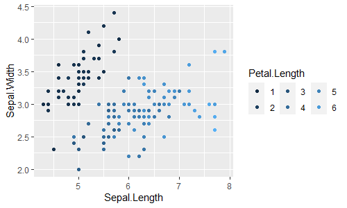
ggplot(data = iris, aes(x = Sepal.Length, y = Sepal.Width)) +
  geom_point(aes(color = Petal.Length)) +
  guides(color = guide_legend(ncol = 3))

ggplot(data = iris, aes(x = Sepal.Length, y = Sepal.Width)) +
  geom_point(aes(color = Petal.Length)) +
  guides(color = guide_legend(ncol = 2, byrow = TRUE))

引数title, title.position：凡例のタイトル

凡例のタイトルの設定です。

R

ggplot(data = iris, aes(x = Sepal.Length, y = Sepal.Width)) +
  geom_point(aes(shape = Species,
                 color = Species,
                 size  = Petal.Width,
                 alpha = Petal.Width)) +
  guides(shape = guide_legend(title = "SPECIES"),
         color = guide_legend(title = "SPECIES"),
         size  = guide_legend(title = "PETAL WIDTH"),
         alpha = guide_legend(title = "PETAL WIDTH"))

ggplot(data = iris, aes(x = Sepal.Length, y = Sepal.Width)) +
  geom_point(aes(color = Species)) +
  guides(color = guide_legend(title = "SPECIES",
                              title.position = "bottom"))

引数label, label.position：凡例のラベル

凡例のラベルの設定です。

R

ggplot(data = iris, aes(x = Sepal.Length, y = Sepal.Width)) +
  geom_point(aes(color = Species)) +
  guides(color = guide_legend(title = "", label = FALSE))

ggplot(data = iris, aes(x = Sepal.Length, y = Sepal.Width)) +
  geom_point(aes(color = Species)) +
  guides(color = guide_legend(label.position = "left"))

ggplot(data = iris, aes(x = Sepal.Length, y = Sepal.Width)) +
  geom_point(aes(color = Species)) +
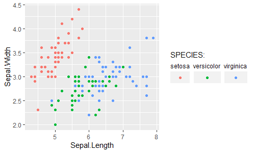
  guides(color = guide_legend(title = "SPECIES:",
                              title.position = "top",
                              label.position = "top",
                              direction = "horizontal"))

ggplot(data = iris, aes(x = Sepal.Length, y = Sepal.Width)) +
  geom_point(aes(color = Species)) +
  guides(color = guide_legend(title = "SPECIES:",
                              title.position = "top",
                              label.position = "top",
                              direction = "horizontal"))

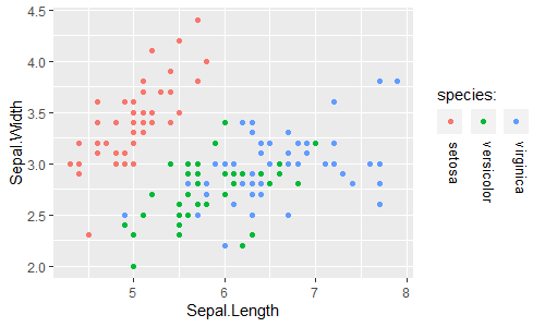
ggplot(data = iris, aes(x = Sepal.Length, y = Sepal.Width)) +
  geom_point(aes(color = Species)) +
  guides(color = guide_legend(title = "species:",
                              title.position = "top",
                              label.position = "bottom",
                              label.hjust = 0,
                              label.vjust = 1,
                              label.theme = element_text(angle = -90, size = 10),
                              direction = "horizontal"))
ggplot(data = iris, aes(x = Sepal.Length, y = Sepal.Width)) +
  geom_point(aes(color = Species)) +
  scale_color_discrete(guide = guide_legend(title = "species:",
                                            title.position = "top",
                                            label.position = "bottom",
                                            label.hjust = 0,
                                            label.vjust = 1,
                                            label.theme = element_text(angle = -90, size = 10),
                                            direction = "horizontal"))

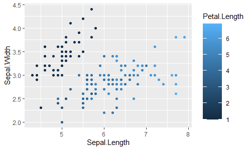
guide_colorbar()：カラーバーを設定する関数

scale_color_continuous(guide = guide_colorbar(... ))とguides(color = guide_colorbar(... ))は同じです。
scale_fill_continuous(guide = guide_colorbar(... ))とguides(fill = guide_colorbar(... ))は同じです。

R

ggplot(data = iris, aes(x = Sepal.Length, y = Sepal.Width)) +
  geom_point(aes(color = Petal.Length))
ggplot(data = iris, aes(x = Sepal.Length, y = Sepal.Width)) +
  geom_point(aes(color = Petal.Length)) +
  scale_color_continuous()
ggplot(data = iris, aes(x = Sepal.Length, y = Sepal.Width)) +
  geom_point(aes(color = Petal.Length)) +
  scale_color_continuous(guide = "colorbar")
ggplot(data = iris, aes(x = Sepal.Length, y = Sepal.Width)) +
  geom_point(aes(color = Petal.Length)) +
  scale_color_continuous(guide = guide_colorbar())
ggplot(data = iris, aes(x = Sepal.Length, y = Sepal.Width)) +
  geom_point(aes(color = Petal.Length)) +
  guides(color = "colorbar")
ggplot(data = iris, aes(x = Sepal.Length, y = Sepal.Width)) +
  geom_point(aes(color = Petal.Length)) +
  guides(color = guide_colorbar())

R

ggplot(data = iris, aes(x = Sepal.Length, y = Sepal.Width)) +
  geom_tile(aes(fill = Petal.Length))
ggplot(data = iris, aes(x = Sepal.Length, y = Sepal.Width)) +
  geom_tile(aes(fill = Petal.Length)) +
  scale_fill_continuous(guide = "colorbar")
ggplot(data = iris, aes(x = Sepal.Length, y = Sepal.Width)) +
  geom_tile(aes(fill = Petal.Length)) +
  scale_fill_continuous(guide = guide_colorbar())
ggplot(data = iris, aes(x = Sepal.Length, y = Sepal.Width)) +
  geom_tile(aes(fill = Petal.Length)) +
  guides(fill = "colorbar")
ggplot(data = iris, aes(x = Sepal.Length, y = Sepal.Width)) +
  geom_tile(aes(fill = Petal.Length)) +
  guides(fill = guide_colorbar())

R

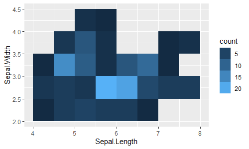
ggplot(data = iris, aes(x = Sepal.Length, y = Sepal.Width)) +
  geom_bin2d(stat = "bin2d", binwidth = 0.5)
ggplot(data = iris, aes(x = Sepal.Length, y = Sepal.Width)) +
  geom_bin2d(stat = "bin2d", binwidth = 0.5) +
  scale_fill_continuous(guide = "colorbar")
ggplot(data = iris, aes(x = Sepal.Length, y = Sepal.Width)) +
  geom_bin2d(stat = "bin2d", binwidth = 0.5) +
  scale_fill_continuous(guide = guide_colorbar())
ggplot(data = iris, aes(x = Sepal.Length, y = Sepal.Width)) +
  geom_bin2d(stat = "bin2d", binwidth = 0.5) +
  guides(fill = "colorbar")
ggplot(data = iris, aes(x = Sepal.Length, y = Sepal.Width)) +
  geom_bin2d(stat = "bin2d", binwidth = 0.5) +
  guides(fill = guide_colorbar())

引数barwidth, barheiht：カラーバーの大きさ

カラーバーの幅と高さの設定です。

R

ggplot(data = iris, aes(x = Sepal.Length, y = Sepal.Width)) +
  geom_point(aes(color = Petal.Length)) +
  guides(color = guide_colorbar(barwidth = 2, barheight = 10))

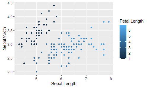
引数ticks, ticks.colour, ticks.linewidth：カラーバーの目盛り

カラーバーの目盛りの設定です。

R

ggplot(data = iris, aes(x = Sepal.Length, y = Sepal.Width)) +
  geom_point(aes(color = Petal.Length)) +
  guides(color = guide_colorbar(ticks = TRUE,            # デフォルト
                                ticks.colour = "white",  # デフォルト
                                ticks.linewidth = 0.5))  # デフォルト

ggplot(data = iris, aes(x = Sepal.Length, y = Sepal.Width)) +
  geom_point(aes(color = Petal.Length)) +
  guides(color = guide_colorbar(ticks = TRUE,
                                ticks.colour = "orange",
                                ticks.linewidth = 3))

ggplot(data = iris, aes(x = Sepal.Length, y = Sepal.Width)) +
  geom_point(aes(color = Petal.Length)) +
  guides(color = guide_colorbar(ticks = FALSE))

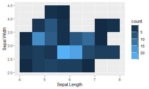
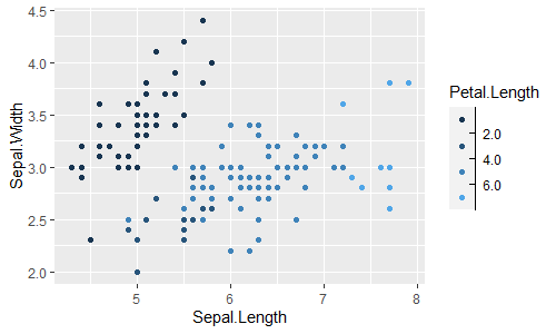
guide_bins()

R

ggplot(data = iris, aes(x = Sepal.Length, y = Sepal.Width)) +
  geom_bin2d(stat = "bin2d", binwidth = 0.5) +
  guides(fill = guide_bins())
ggplot(data = iris, aes(x = Sepal.Length, y = Sepal.Width)) +
  geom_bin2d(stat = "bin2d", binwidth = 0.5) +
  guides(fill = "bins")

R

ggplot(data = iris, aes(x = Sepal.Length, y = Sepal.Width)) +
  geom_point(aes(color = Petal.Length)) +
  scale_color_binned(breaks = c(2, 4, 6)) +
  guides(color = "bins")
ggplot(data = iris, aes(x = Sepal.Length, y = Sepal.Width)) +
  geom_point(aes(color = Petal.Length)) +
  scale_color_binned(breaks = c(2, 4, 6)) +
  guides(color = guide_bins())

guide_coloursteps()

R

ggplot(data = iris, aes(x = Sepal.Length, y = Sepal.Width)) +
  geom_point(aes(color = Petal.Length)) +
  scale_color_binned(breaks = c(2, 4, 6))
ggplot(data = iris, aes(x = Sepal.Length, y = Sepal.Width)) +
  geom_point(aes(color = Petal.Length)) +
  scale_color_binned(breaks = c(2, 4, 6)) +
  guides(color = "coloursteps")
ggplot(data = iris, aes(x = Sepal.Length, y = Sepal.Width)) +
  geom_point(aes(color = Petal.Length)) +
  scale_color_binned(breaks = c(2, 4, 6)) +
  guides(color = guide_coloursteps())

引数even.steps

R

ggplot(data = iris, aes(x = Sepal.Length, y = Sepal.Width)) +
  geom_point(aes(color = Petal.Length)) +
  scale_color_binned(breaks = c(2, 3, 5),
                     guide = guide_colorsteps())
ggplot(data = iris, aes(x = Sepal.Length, y = Sepal.Width)) +
  geom_point(aes(color = Petal.Length)) +
  scale_color_binned(breaks = c(2, 3, 5),
                     guide = "coloursteps")
ggplot(data = iris, aes(x = Sepal.Length, y = Sepal.Width)) +
  geom_point(aes(color = Petal.Length)) +
  scale_color_binned(breaks = c(2, 3, 5)) +
  guides(color = "coloursteps")
ggplot(data = iris, aes(x = Sepal.Length, y = Sepal.Width)) +
  geom_point(aes(color = Petal.Length)) +
  scale_color_binned(breaks = c(2, 3, 5)) +
  guides(color = guide_colorsteps())

ggplot(data = iris, aes(x = Sepal.Length, y = Sepal.Width)) +
  geom_point(aes(color = Petal.Length)) +
  scale_color_binned(breaks = c(2, 3, 5),
                     guide = guide_colorsteps(even.steps = FALSE))
ggplot(data = iris, aes(x = Sepal.Length, y = Sepal.Width)) +
  geom_point(aes(color = Petal.Length)) +
  scale_color_binned(breaks = c(2, 3, 5)) +
  guides(color = guide_colorsteps(even.steps = FALSE))

ggplot(data = iris, aes(x = Sepal.Length, y = Sepal.Width)) +
  geom_point(aes(color = Petal.Length)) +
  scale_color_binned(breaks = c(2, 3, 5),
                     guide = guide_colorsteps(show.limits = TRUE, even.steps = FALSE))
ggplot(data = iris, aes(x = Sepal.Length, y = Sepal.Width)) +
  geom_point(aes(color = Petal.Length)) +
  scale_color_binned(breaks = c(2, 3, 5)) +
  guides(color = guide_colorsteps(show.limits = TRUE, even.steps = FALSE))

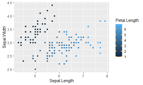
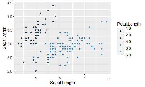
引数show.limits

R

ggplot(data = iris, aes(x = Sepal.Length, y = Sepal.Width)) +
  geom_point(aes(color = Petal.Length)) +
  scale_color_binned(breaks = c(2, 4, 6),
                     guide= guide_bins())
ggplot(data = iris, aes(x = Sepal.Length, y = Sepal.Width)) +
  geom_point(aes(color = Petal.Length)) +
  scale_color_binned(breaks = c(2, 4, 6)) +
  guides(color = guide_bins())

ggplot(data = iris, aes(x = Sepal.Length, y = Sepal.Width)) +
  geom_point(aes(color = Petal.Length)) +
  scale_color_binned(breaks = c(2, 4, 6),
                     guide = guide_bins(show.limits = TRUE))
ggplot(data = iris, aes(x = Sepal.Length, y = Sepal.Width)) +
  geom_point(aes(color = Petal.Length)) +
  scale_color_binned(breaks = c(2, 4, 6)) +
  guides(color = guide_bins(show.limits = TRUE))

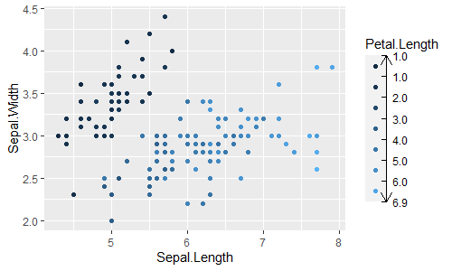
引数axis.arrow

R

ggplot(data = iris, aes(x = Sepal.Length, y = Sepal.Width)) +
  geom_point(aes(color = Petal.Length)) +
  guides(color = guide_bins(axis.arrow = arrow(length = unit(0.5, "npc"), ends = "both"),
                            show.limits = TRUE))

ggplot(data = iris, aes(x = Sepal.Length, y = Sepal.Width)) +
  geom_point(aes(color = Petal.Length)) +
  theme(legend.position = "bottom") +
  guides(color = guide_bins(axis.arrow = arrow(length = unit(0.5, "npc"), ends = "both"),
                            show.limits = TRUE))

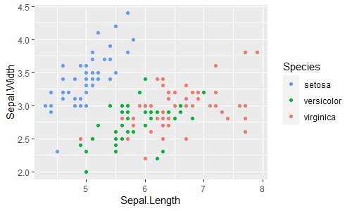
scale_*_manual()：離散値のcolor軸などの手動設定

scale_*_discrete()ではcolorなどが自動的に割り振られますが、これを直接手動（マニュアル）で設定したい場合にはscale_*_manual()を使います。

引数values：手動設定したい値の指定

valuesに設定したい値からなるベクトルを与えることで設定します。
名前付きベクトルの形で与えると、名前に対してベクトルの値が設定されます。

R

c("setosa" = "red", "versicolor" = "green", "virginica" = "blue")
#     setosa versicolor  virginica 
#      "red"    "green"     "blue"

ggplot(data = iris, aes(x = Sepal.Length, y = Sepal.Width)) +
  geom_point(aes(color = Species)) +
  scale_color_manual(values = c("red", "green", "blue"))
ggplot(data = iris, aes(x = Sepal.Length, y = Sepal.Width)) +
  geom_point(aes(color = Species)) +
  scale_color_manual(values = c("setosa"     = "red",
                                "versicolor" = "green",
                                "virginica"  = "blue"))
ggplot(data = iris, aes(x = Sepal.Length, y = Sepal.Width)) +
  geom_point(aes(color = Species)) +
  scale_color_manual(values = c("setosa"     = 2,  # red
                                "versicolor" = 3,  # green
                                "virginica"  = 4)) # blue
ggplot(data = iris, aes(x = Sepal.Length, y = Sepal.Width)) +
  geom_point(aes(color = Species)) +
  scale_color_manual(values = c("versicolor" = "green",
                                "virginica"  = "blue",
                                "setosa"     = "red"))

R

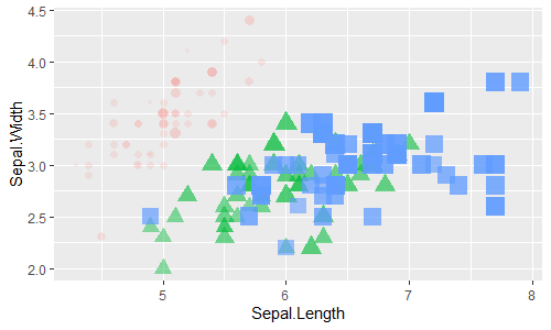
ggplot(data = iris, aes(x = Sepal.Length, y = Sepal.Width)) +
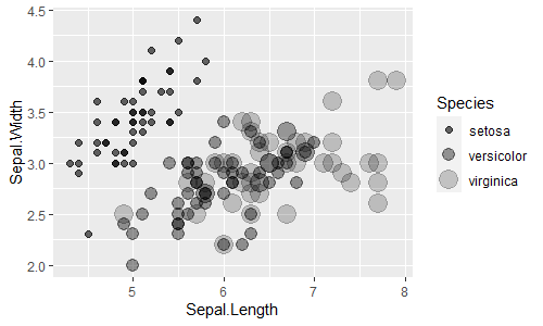
  geom_point(aes(alpha = Species, size = Species)) +
  scale_alpha_manual(values = c("setosa"     = 3/5,
                                "versicolor" = 2/5,
                                "virginica"  = 1/5)) +
  scale_size_manual(values = c("setosa"     = 2,
                               "versicolor" = 4,
                               "virginica"  = 6))

R

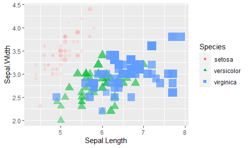
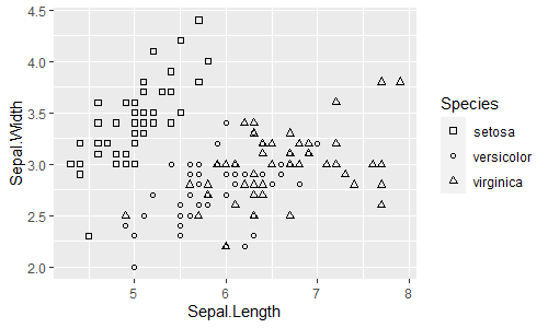
ggplot(data = iris, aes(x = Sepal.Length, y = Sepal.Width)) +
  geom_point(aes(shape = Species)) +
  scale_shape_manual(values = c("setosa"     = 0,
                                "versicolor" = 1,
                                "virginica"  = 2))

R

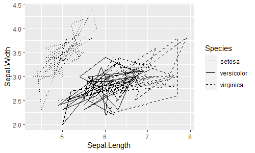
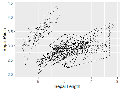
ggplot(data = iris, aes(x = Sepal.Length, y = Sepal.Width)) +
  geom_path(aes(linetype = Species)) +
  scale_linetype_manual(values = c("setosa"     = "dotted",
                                   "versicolor" = "solid",
                                   "virginica"  = "dashed"))

scale_*_identity()：color軸などのデータの値をそのまま設定

scale_*_discrete()ではcolorなどが自動的に割り振られますが、これをデータの値そのままに設定したい場合にはscale_*_identity()を使います。

まず、データを用意しておきます。irisデータに次の列を追加しています。
・col列：color軸に設定したい色
・lty列：linetype軸に設定したい線の種類
・s列 ：size軸に設定したいサイズ
・a列 ：alpha軸に設定したい透過度

R

iris_2 <- iris %>% as_tibble() %>% 
  mutate(col = case_when(Species == "setosa"     ~ "red",
                         Species == "versicolor" ~ "green",
                         Species == "virginica"  ~ "blue"),
         lty = case_when(Species == "setosa"     ~ "dotted",
                         Species == "versicolor" ~ "solid",
                         Species == "virginica"  ~ "dashed"),
         s = round(Petal.Length),
         a = (8 - s) / 10) %>% 
  print()
# # A tibble: 150 x 9
#    Sepal.Length Sepal.Width Petal.Length Petal.Width Species col   lty        s     a
#           <dbl>       <dbl>        <dbl>       <dbl> <fct>   <chr> <chr>  <dbl> <dbl>
#  1          5.1         3.5          1.4         0.2 setosa  red   dotted     1   0.7
#  2          4.9         3            1.4         0.2 setosa  red   dotted     1   0.7
#  3          4.7         3.2          1.3         0.2 setosa  red   dotted     1   0.7
#  4          4.6         3.1          1.5         0.2 setosa  red   dotted     2   0.6
#  5          5           3.6          1.4         0.2 setosa  red   dotted     1   0.7
#  6          5.4         3.9          1.7         0.4 setosa  red   dotted     2   0.6
#  7          4.6         3.4          1.4         0.3 setosa  red   dotted     1   0.7
#  8          5           3.4          1.5         0.2 setosa  red   dotted     2   0.6
#  9          4.4         2.9          1.4         0.2 setosa  red   dotted     1   0.7
# 10          4.9         3.1          1.5         0.1 setosa  red   dotted     2   0.6
# # ... with 140 more rows

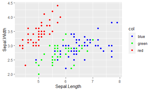
color軸の変数に色の値が入ったcol列を指定してscale_color_identity()を使います。
なお、scale_color_identity()はデフォルトでguide = "none"（凡例を表示しない）ですので、guide = "legend"として凡例を表示しています。
また、geom_point(aes(color = col)) + scale_color_identity()は、geom_point(aes(color = I(col)))と同じです。このI()はcol列の値をそのままcolor軸に設定する（identity）ものです。
変数としてaesに入れずに、geom_point()の引数colorにデータと同じ個数の値を指定しても同じです（color = iris_2$col）。

R

ggplot(data = iris_2, aes(x = Sepal.Length, y = Sepal.Width)) +
  geom_point(aes(color = col)) +
  scale_color_identity(guide = "legend")

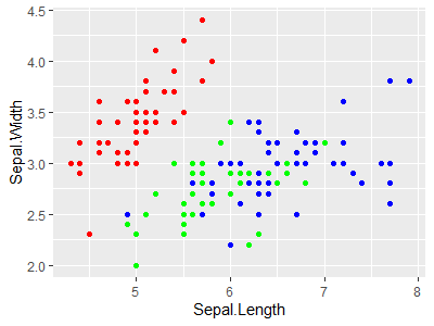
ggplot(data = iris_2, aes(x = Sepal.Length, y = Sepal.Width)) +
  geom_point(aes(color = col)) +
  scale_color_identity(guide = "none")  # デフォルト
ggplot(data = iris_2, aes(x = Sepal.Length, y = Sepal.Width)) +
  geom_point(aes(color = col)) +
  scale_color_identity()
ggplot(data = iris_2, aes(x = Sepal.Length, y = Sepal.Width)) +
  geom_point(aes(color = I(col)))
ggplot(data = iris_2, aes(x = Sepal.Length, y = Sepal.Width)) +
  geom_point(color = iris_2$col)

R

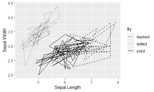
ggplot(data = iris_2, aes(x = Sepal.Length, y = Sepal.Width)) +
  geom_path(aes(linetype = lty)) +
  scale_linetype_identity(guide = "legend")

ggplot(data = iris_2, aes(x = Sepal.Length, y = Sepal.Width)) +
  geom_path(aes(linetype = lty)) +
  scale_linetype_identity(guide = "none")
ggplot(data = iris_2, aes(x = Sepal.Length, y = Sepal.Width)) +
  geom_path(aes(linetype = lty)) +
  scale_linetype_identity()
ggplot(data = iris_2, aes(x = Sepal.Length, y = Sepal.Width)) +
  geom_path(aes(linetype = I(lty)))
# ggplot(data = iris_2, aes(x = Sepal.Length, y = Sepal.Width)) +
#   geom_path(linetype = iris_2$lty)

R

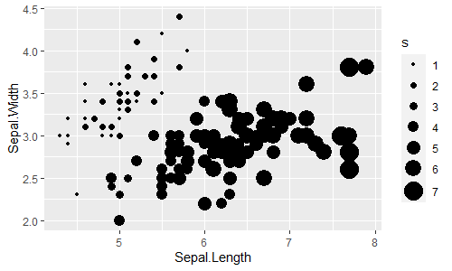
ggplot(data = iris_2, aes(x = Sepal.Length, y = Sepal.Width)) +
  geom_point(aes(size = s)) +
  scale_size_identity(guide = "legend")

ggplot(data = iris_2, aes(x = Sepal.Length, y = Sepal.Width)) +
  geom_point(aes(size = s)) +
  scale_size_identity(guide = "none")
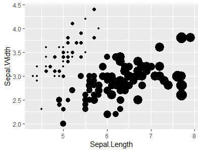
ggplot(data = iris_2, aes(x = Sepal.Length, y = Sepal.Width)) +
  geom_point(aes(size = s)) +
  scale_size_identity()
ggplot(data = iris_2, aes(x = Sepal.Length, y = Sepal.Width)) +
  geom_point(aes(size = I(s)))
ggplot(data = iris_2, aes(x = Sepal.Length, y = Sepal.Width)) +
  geom_point(size = iris_2$s)

R

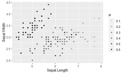
ggplot(data = iris_2, aes(x = Sepal.Length, y = Sepal.Width)) +
  geom_point(aes(alpha = a)) +
  scale_alpha_identity(guide = "legend")

ggplot(data = iris_2, aes(x = Sepal.Length, y = Sepal.Width)) +
  geom_point(aes(alpha = a)) +
  scale_alpha_identity(guide = "none")
ggplot(data = iris_2, aes(x = Sepal.Length, y = Sepal.Width)) +
  geom_point(aes(alpha = a)) +
  scale_alpha_identity()
ggplot(data = iris_2, aes(x = Sepal.Length, y = Sepal.Width)) +
  geom_point(aes(alpha = I(a)))
ggplot(data = iris_2, aes(x = Sepal.Length, y = Sepal.Width)) +
  geom_point(alpha = iris_2$a)

scale_color_*(), scale_fill_*()：color軸, fill軸

引数nameは共通して使えます。

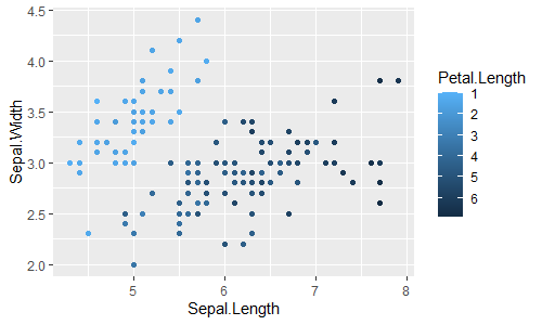
色を反転するには、scale_*_gradient()のように色を直接指定するものは指定する色を反転すればよく、scale_*_distiller()のようにカラーパレットを指定するものはdirection = -1で反転できます。また、scale_*_continuous()等はtrans = "reverse"で反転できます。

scale_color_gradient(), scale_fill_gradient()：連続値のcolor軸, fill軸

scale_color_steps(), scale_fill_steps()：連続値のcolor軸, fill軸のビン分割

2色 (low-high) のグラデーションの色スケールです。

• scale_*_gradient()：連続値のcolor軸, fill軸をグラデーションで
• scale_*_steps()：連続値のcolor軸, fill軸をビン分割してグラデーションで

R

ggplot(data = iris, aes(x = Sepal.Length, y = Sepal.Width)) +
  geom_point(aes(color = Petal.Length))
ggplot(data = iris, aes(x = Sepal.Length, y = Sepal.Width)) +
  geom_point(aes(color = Petal.Length)) +
  scale_color_gradient()
ggplot(data = iris, aes(x = Sepal.Length, y = Sepal.Width)) +
  geom_point(aes(color = Petal.Length)) +
  scale_color_gradient(low = "#132B43", high = "#56B1F7")  # デフォルト

ggplot(data = iris, aes(x = Sepal.Length, y = Sepal.Width)) +
  geom_point(aes(color = Petal.Length)) +
  scale_color_gradient(low = "#56B1F7", high = "#132B43")

ggplot(data = iris, aes(x = Sepal.Length, y = Sepal.Width)) +
  geom_point(aes(color = Petal.Length)) +
  scale_color_gradient(low = "green", high = "red")

R

ggplot(data = iris, aes(x = Sepal.Length, y = Sepal.Width)) +
  geom_point(aes(color = Petal.Length)) +
  scale_color_steps()
ggplot(data = iris, aes(x = Sepal.Length, y = Sepal.Width)) +
  geom_point(aes(color = Petal.Length)) +
  scale_color_steps(low = "#132B43", high = "#56B1F7")  # デフォルト

ggplot(data = iris, aes(x = Sepal.Length, y = Sepal.Width)) +
  geom_point(aes(color = Petal.Length)) +
  scale_color_steps(low = "green", high = "red")

R

ggplot(data = iris, aes(x = Sepal.Length, y = Sepal.Width)) +
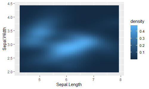
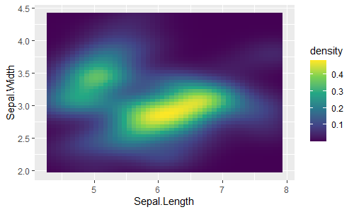
  geom_tile(stat = "density_2d", contour = FALSE, n = 50, aes(fill = ..density..))
ggplot(data = iris, aes(x = Sepal.Length, y = Sepal.Width)) +
  geom_tile(stat = "density_2d", contour = FALSE, n = 50, aes(fill = ..density..)) +
  scale_fill_gradient()

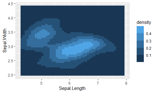
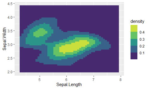
ggplot(data = iris, aes(x = Sepal.Length, y = Sepal.Width)) +
  geom_tile(stat = "density_2d", contour = FALSE, n = 50, aes(fill = ..density..)) +
  scale_fill_steps()

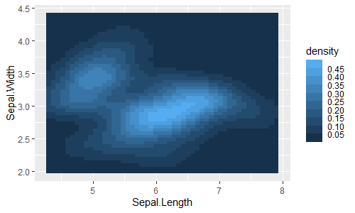
ggplot(data = iris, aes(x = Sepal.Length, y = Sepal.Width)) +
  geom_tile(stat = "density_2d", contour = FALSE, n = 50, aes(fill = ..density..)) +
  scale_fill_steps(breaks = seq(0, 0.5, by = 0.05))

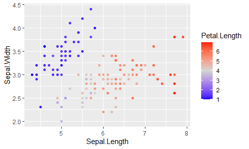
scale_color_gradient2(), scale_fill_gradient2()：連続値のcolor軸, fill軸

scale_color_steps2(), scale_fill_steps2()：連続値のcolor軸, fill軸のビン分割

3色 (low-mid-high) のグラデーションの色スケールです。

• scale_*_gradient2()：連続値のcolor軸, fill軸をグラデーションで
• scale_*_steps2()：連続値のcolor軸, fill軸をビン分割してグラデーションで

R

ggplot(data = iris, aes(x = Sepal.Length, y = Sepal.Width)) +
  geom_point(aes(color = Petal.Length)) +
  scale_color_gradient2(low = "blue", mid = "lightgray", high = "red",
                        midpoint = 4)

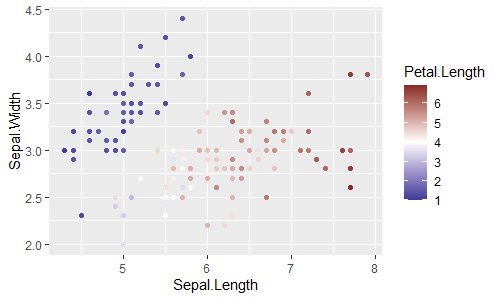
library(scales)
ggplot(data = iris, aes(x = Sepal.Length, y = Sepal.Width)) +
  geom_point(aes(color = Petal.Length)) +
  scale_color_gradient2(low = muted("blue"), mid = "white", high = muted("red"),
                        midpoint = 4)

R

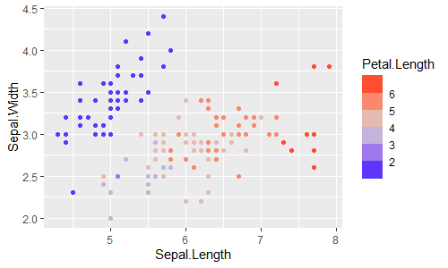
ggplot(data = iris, aes(x = Sepal.Length, y = Sepal.Width)) +
  geom_point(aes(color = Petal.Length)) +
  scale_color_steps2(low = "blue", mid = "lightgray", high = "red",
                     midpoint = 4)

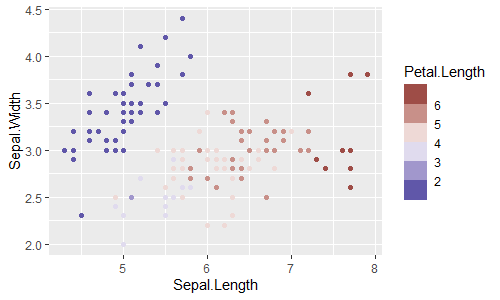
library(scales)
ggplot(data = iris, aes(x = Sepal.Length, y = Sepal.Width)) +
  geom_point(aes(color = Petal.Length)) +
  scale_color_steps2(low = muted("blue"), mid = "white", high = muted("red"),
                     midpoint = 4)

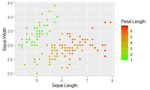
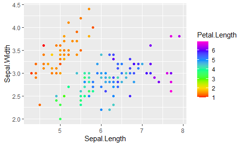
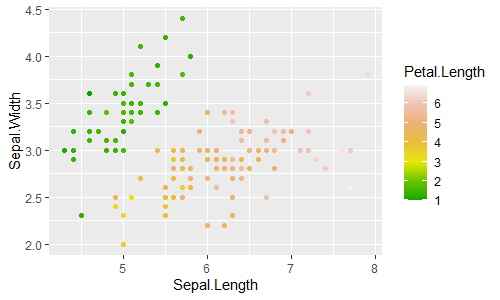
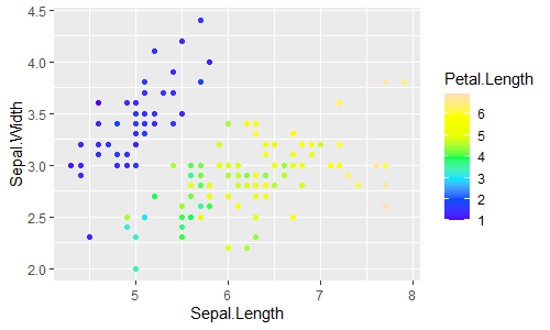
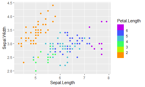
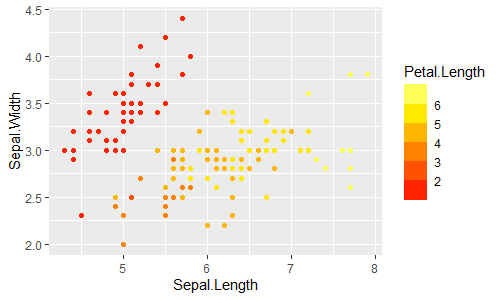
scale_color_gradientn(), scale_fill_gradientn()：連続値のcolor軸, fill軸

scale_color_stepsn(), scale_fill_stepsn()：連続値のcolor軸, fill軸のビン分割

n色のグラデーションの色スケールです。

• scale_*_gradientn()：連続値のcolor軸, fill軸をグラデーションで
• scale_*_stepsn()：連続値のcolor軸, fill軸をビン分割してグラデーションで

R

ggplot(data = iris, aes(x = Sepal.Length, y = Sepal.Width)) +
  geom_point(aes(color = Petal.Length)) +
  scale_color_gradientn(colors = rainbow(7))

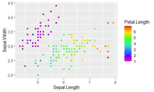
ggplot(data = iris, aes(x = Sepal.Length, y = Sepal.Width)) +
  geom_point(aes(color = Petal.Length)) +
  scale_color_gradientn(colors = rev(rainbow(7)))

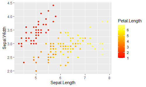
ggplot(data = iris, aes(x = Sepal.Length, y = Sepal.Width)) +
  geom_point(aes(color = Petal.Length)) +
  scale_color_gradientn(colors = heat.colors(7))

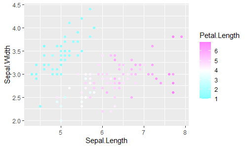
ggplot(data = iris, aes(x = Sepal.Length, y = Sepal.Width)) +
  geom_point(aes(color = Petal.Length)) +
  scale_color_gradientn(colors = cm.colors(7))

ggplot(data = iris, aes(x = Sepal.Length, y = Sepal.Width)) +
  geom_point(aes(color = Petal.Length)) +
  scale_color_gradientn(colors = terrain.colors(7))

ggplot(data = iris, aes(x = Sepal.Length, y = Sepal.Width)) +
  geom_point(aes(color = Petal.Length)) +
  scale_color_gradientn(colors = topo.colors(7))

R

ggplot(data = iris, aes(x = Sepal.Length, y = Sepal.Width)) +
  geom_point(aes(color = Petal.Length)) +
  scale_color_stepsn(colors = rainbow(7))

ggplot(data = iris, aes(x = Sepal.Length, y = Sepal.Width)) +
  geom_point(aes(color = Petal.Length)) +
  scale_color_stepsn(colors = heat.colors(7))

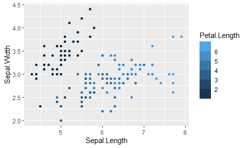
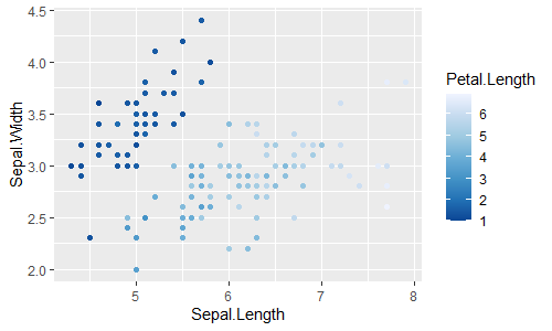
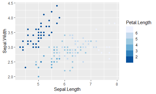
scale_color_distiller(), scale_fill_distiller()：連続値のcolor軸, fill軸

scale_color_fermenter(), scale_fill_fermenter()：連続値のcolor軸, fill軸のビン分割

• scale_*_distiller()：連続値のcolor軸, fill軸をColorBrewerのパレットで
• scale_*_fermenter()：連続値のcolor軸, fill軸をビン分割してColorBrewerのパレットで

R

ggplot(data = iris, aes(x = Sepal.Length, y = Sepal.Width)) +
  geom_point(aes(color = Petal.Length)) +
  scale_color_distiller()
ggplot(data = iris, aes(x = Sepal.Length, y = Sepal.Width)) +
  geom_point(aes(color = Petal.Length)) +
  scale_color_distiller(palette = "Blues")  # デフォルト
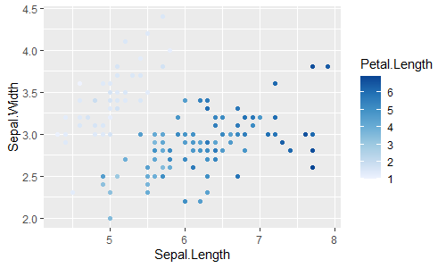
ggplot(data = iris, aes(x = Sepal.Length, y = Sepal.Width)) +
  geom_point(aes(color = Petal.Length)) +
  scale_color_distiller(palette = "Blues", direction = -1)  # デフォルト

ggplot(data = iris, aes(x = Sepal.Length, y = Sepal.Width)) +
  geom_point(aes(color = Petal.Length)) +
  scale_color_distiller(palette = "Blues", direction = 1)

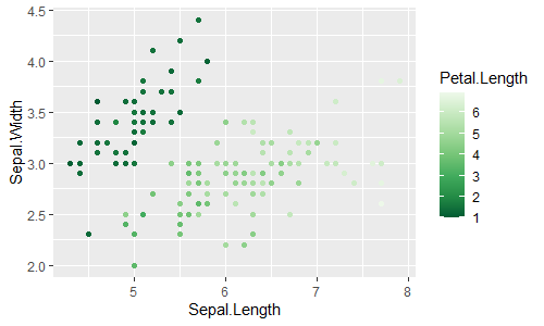
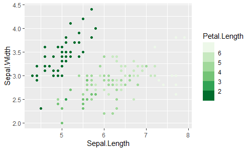
ggplot(data = iris, aes(x = Sepal.Length, y = Sepal.Width)) +
  geom_point(aes(color = Petal.Length)) +
  scale_color_distiller(palette = "Greens")

ggplot(data = iris, aes(x = Sepal.Length, y = Sepal.Width)) +
  geom_point(aes(color = Petal.Length)) +
  scale_color_distiller(palette = "Set1")

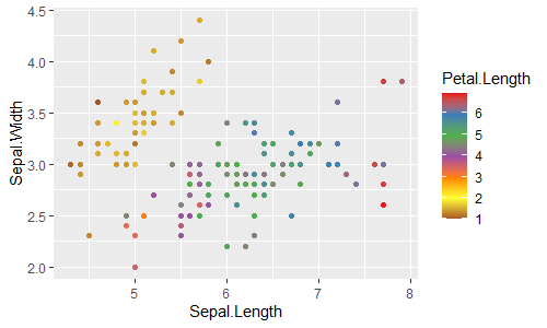
ggplot(data = iris, aes(x = Sepal.Length, y = Sepal.Width)) +
  geom_point(aes(color = Petal.Length)) +
  scale_color_distiller(palette = "Spectral")

R

ggplot(data = iris, aes(x = Sepal.Length, y = Sepal.Width)) +
  geom_point(aes(color = Petal.Length)) +
  scale_color_fermenter()
ggplot(data = iris, aes(x = Sepal.Length, y = Sepal.Width)) +
  geom_point(aes(color = Petal.Length)) +
  scale_color_fermenter(palette = "Blues")
ggplot(data = iris, aes(x = Sepal.Length, y = Sepal.Width)) +
  geom_point(aes(color = Petal.Length)) +
  scale_color_fermenter(palette = "Blues", direction = -1)

ggplot(data = iris, aes(x = Sepal.Length, y = Sepal.Width)) +
  geom_point(aes(color = Petal.Length)) +
  scale_color_fermenter(palette = "Greens")

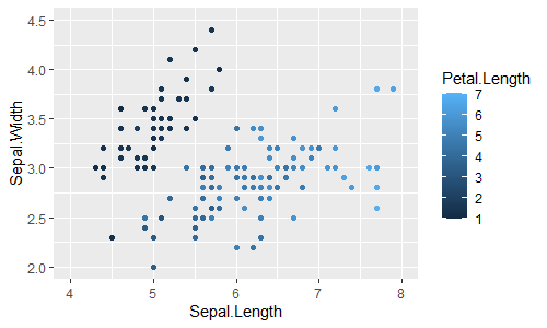
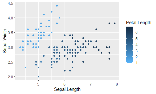
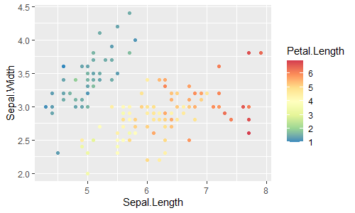
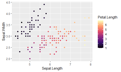
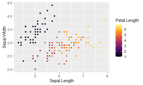
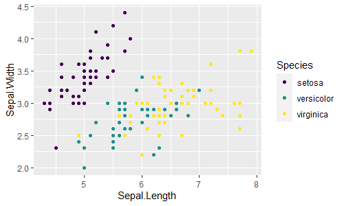
scale_color_continuous(), scale_fill_continuous()：連続値のcolor軸, fill軸

scale_color_binned(), scale_fill_binned()：連続値のcolor軸, fill軸のビン分割

R

ggplot(data = iris, aes(x = Sepal.Length, y = Sepal.Width)) +
  geom_point(aes(color = Petal.Length))
ggplot(data = iris, aes(x = Sepal.Length, y = Sepal.Width)) +
  geom_point(aes(color = Petal.Length)) +
  scale_color_continuous()
ggplot(data = iris, aes(x = Sepal.Length, y = Sepal.Width)) +
  geom_point(aes(color = Petal.Length)) +
  scale_color_continuous(type = "gradient")  # デフォルト

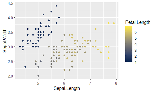
ggplot(data = iris, aes(x = Sepal.Length, y = Sepal.Width)) +
  geom_point(aes(color = Petal.Length)) +
  scale_color_continuous(type = "viridis")
ggplot(data = iris, aes(x = Sepal.Length, y = Sepal.Width)) +
  geom_point(aes(color = Petal.Length)) +
  scale_color_viridis_c()

R

ggplot(data = iris, aes(x = Sepal.Length, y = Sepal.Width)) +
  geom_point(aes(color = Petal.Length)) +
  scale_color_binned(type = "gradient")

ggplot(data = iris, aes(x = Sepal.Length, y = Sepal.Width)) +
  geom_point(aes(color = Petal.Length)) +
  scale_color_binned(type = "viridis")
ggplot(data = iris, aes(x = Sepal.Length, y = Sepal.Width)) +
  geom_point(aes(color = Petal.Length)) +
  scale_colour_viridis_b()
# ggplot(data = iris, aes(x = Sepal.Length, y = Sepal.Width)) +
#   geom_point(aes(color = Petal.Length)) +
#   scale_color_viridis_b()

注）scale_color_viridis_c()とscale_color_viridis_d()はあるが、scale_color_viridis_b()だけなぜか定義されていない。

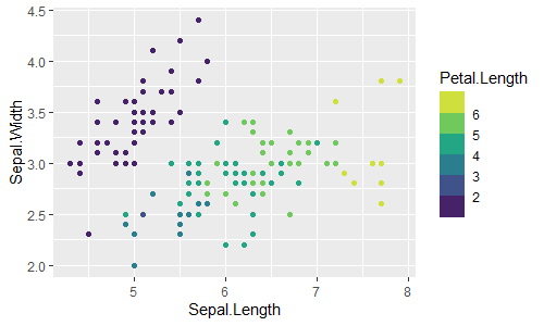
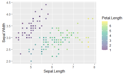
scale_color_viridis_c(), scale_fill_viridis_c()：連続値のcolor軸, fill軸

scale_colour_viridis_b(), scale_fill_viridis_b()：連続値のcolor軸, fill軸のビン分割

• scale_*_viridis_c()：連続値のcolor軸, fill軸をviridisLiteのパレットで
• scale_*_viridis_b()：連続値のcolor軸, fill軸をビン分割してviridisLiteのパレットで

R

ggplot(data = iris, aes(x = Sepal.Length, y = Sepal.Width)) +
  geom_point(aes(color = Petal.Length)) +
  scale_color_viridis_c()
ggplot(data = iris, aes(x = Sepal.Length, y = Sepal.Width)) +
  geom_point(aes(color = Petal.Length)) +
  scale_color_viridis_c(option = "D")  # デフォルト
ggplot(data = iris, aes(x = Sepal.Length, y = Sepal.Width)) +
  geom_point(aes(color = Petal.Length)) +
  scale_color_viridis_c(option = "viridis")  # デフォルト

ggplot(data = iris, aes(x = Sepal.Length, y = Sepal.Width)) +
  geom_point(aes(color = Petal.Length)) +
  scale_color_viridis_c(option = "A")
ggplot(data = iris, aes(x = Sepal.Length, y = Sepal.Width)) +
  geom_point(aes(color = Petal.Length)) +
  scale_color_viridis_c(option = "magma")

ggplot(data = iris, aes(x = Sepal.Length, y = Sepal.Width)) +
  geom_point(aes(color = Petal.Length)) +
  scale_color_viridis_c(option = "B")
ggplot(data = iris, aes(x = Sepal.Length, y = Sepal.Width)) +
  geom_point(aes(color = Petal.Length)) +
  scale_color_viridis_c(option = "inferno")

ggplot(data = iris, aes(x = Sepal.Length, y = Sepal.Width)) +
  geom_point(aes(color = Petal.Length)) +
  scale_color_viridis_c(option = "C")
ggplot(data = iris, aes(x = Sepal.Length, y = Sepal.Width)) +
  geom_point(aes(color = Petal.Length)) +
  scale_color_viridis_c(option = "plasma")

ggplot(data = iris, aes(x = Sepal.Length, y = Sepal.Width)) +
  geom_point(aes(color = Petal.Length)) +
  scale_color_viridis_c(option = "E")
ggplot(data = iris, aes(x = Sepal.Length, y = Sepal.Width)) +
  geom_point(aes(color = Petal.Length)) +
  scale_color_viridis_c(option = "cividis")

ggplot(data = iris, aes(x = Sepal.Length, y = Sepal.Width)) +
  geom_point(aes(color = Petal.Length)) +
  scale_color_viridis_c(alpha = 0.5)

ggplot(data = iris, aes(x = Sepal.Length, y = Sepal.Width)) +
  geom_point(aes(color = Petal.Length)) +
  scale_color_viridis_c(direction = -1)

R

ggplot(data = iris, aes(x = Sepal.Length, y = Sepal.Width)) +
  geom_point(aes(color = Petal.Length)) +
  scale_colour_viridis_b()
ggplot(data = iris, aes(x = Sepal.Length, y = Sepal.Width)) +
  geom_point(aes(color = Petal.Length)) +
  scale_colour_viridis_b(option = "D")  # デフォルト

注）scale_color_viridis_c()とscale_color_viridis_d()はあるが、scale_color_viridis_b()だけなぜか定義されていない²。

R

ggplot(data = iris, aes(x = Sepal.Length, y = Sepal.Width)) +
  geom_tile(stat = "density_2d", contour = FALSE, n = 50, aes(fill = ..density..)) +
  scale_fill_viridis_c()

ggplot(data = iris, aes(x = Sepal.Length, y = Sepal.Width)) +
  geom_tile(stat = "density_2d", contour = FALSE, n = 50, aes(fill = ..density..)) +
  scale_fill_viridis_b()

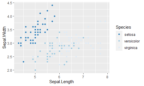
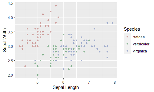
scale_color_brewer(), scale_fill_brewer()：離散値のcolor軸, fill軸

R

ggplot(data = iris, aes(x = Sepal.Length, y = Sepal.Width)) +
  geom_point(aes(color = Species)) +
  scale_color_brewer()
ggplot(data = iris, aes(x = Sepal.Length, y = Sepal.Width)) +
  geom_point(aes(color = Species)) +
  scale_color_brewer()
ggplot(data = iris, aes(x = Sepal.Length, y = Sepal.Width)) +
  geom_point(aes(color = Species)) +
  scale_color_brewer(palette = "Blues")
ggplot(data = iris, aes(x = Sepal.Length, y = Sepal.Width)) +
  geom_point(aes(color = Species)) +
  scale_color_brewer(palette = 1)
ggplot(data = iris, aes(x = Sepal.Length, y = Sepal.Width)) +
  geom_point(aes(color = Species)) +
  scale_color_brewer(palette = 1, direction = 1)

ggplot(data = iris, aes(x = Sepal.Length, y = Sepal.Width)) +
  geom_point(aes(color = Species)) +
  scale_color_brewer(palette = "Blues", direction = -1)

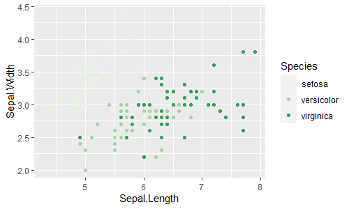
ggplot(data = iris, aes(x = Sepal.Length, y = Sepal.Width)) +
  geom_point(aes(color = Species)) +
  scale_color_brewer(palette = "Greens")

ggplot(data = iris, aes(x = Sepal.Length, y = Sepal.Width)) +
  geom_point(aes(color = Species)) +
  scale_color_brewer(palette = "Set1")

ggplot(data = iris, aes(x = Sepal.Length, y = Sepal.Width)) +
  geom_point(aes(color = Species)) +
  scale_color_brewer(palette = "Set2")

ggplot(data = iris, aes(x = Sepal.Length, y = Sepal.Width)) +
  geom_point(aes(color = Species)) +
  scale_color_brewer(palette = "Set3")

ggplot(data = iris, aes(x = Sepal.Length, y = Sepal.Width)) +
  geom_point(aes(color = Species)) +
  scale_color_brewer(palette = "Accent")

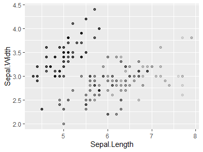
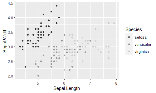
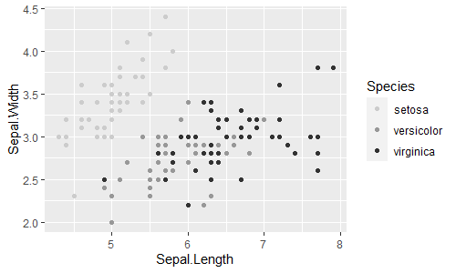
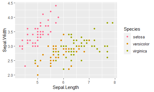
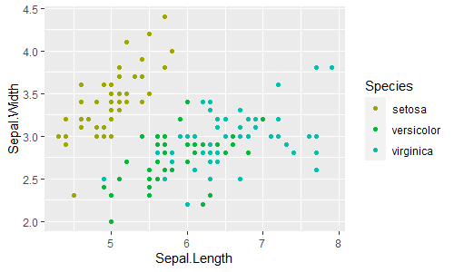
scale_color_grey(), scale_fill_grey()：離散値のcolor軸, fill軸

• scale_*_grey()：離散値のcolor軸, fill軸をグレースケールで

R

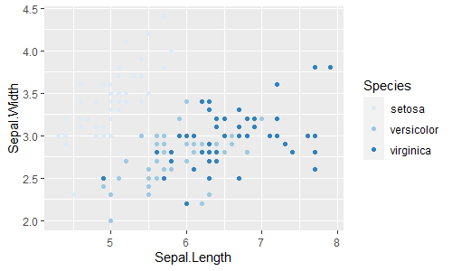
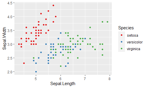
ggplot(data = iris, aes(x = Sepal.Length, y = Sepal.Width)) +
  geom_point(aes(color = Species)) +
  scale_color_grey()
ggplot(data = iris, aes(x = Sepal.Length, y = Sepal.Width)) +
  geom_point(aes(color = Species)) +
  scale_color_grey(start = 0.2, end = 0.8)  # デフォルト

ggplot(data = iris, aes(x = Sepal.Length, y = Sepal.Width)) +
  geom_point(aes(color = Species)) +
  scale_color_grey(start = 0.8, end = 0.2)

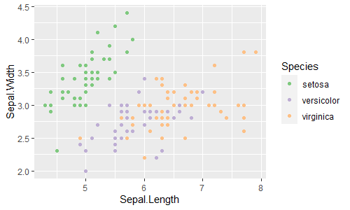
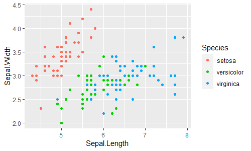
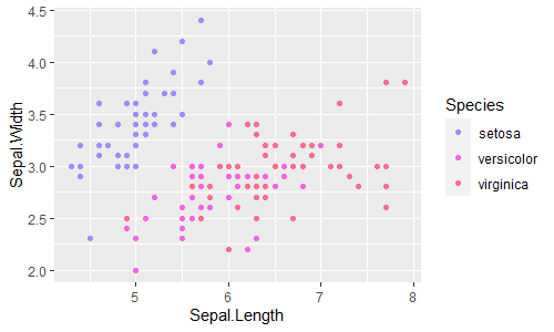
scale_color_hue(), scale_fill_hue()：離散値のcolor軸, fill軸

• scale_*_hue()：離散値のcolor軸, fill軸をデフォルト色スケールで

R

ggplot(data = iris, aes(x = Sepal.Length, y = Sepal.Width)) +
  geom_point(aes(color = Species))
ggplot(data = iris, aes(x = Sepal.Length, y = Sepal.Width)) +
  geom_point(aes(color = Species)) +
  scale_color_hue()
ggplot(data = iris, aes(x = Sepal.Length, y = Sepal.Width)) +
  geom_point(aes(color = Species)) +
  scale_color_hue(h = c(0, 360) + 15,
                  c = 100,
                  l = 65,
                  direction = 1)  # デフォルト

ggplot(data = iris, aes(x = Sepal.Length, y = Sepal.Width)) +
  geom_point(aes(color = Species)) +
  scale_color_hue(direction = -1)

ggplot(data = iris, aes(x = Sepal.Length, y = Sepal.Width)) +
  geom_point(aes(color = Species)) +
  scale_color_hue(l = 40, c = 30)

ggplot(data = iris, aes(x = Sepal.Length, y = Sepal.Width)) +
  geom_point(aes(color = Species)) +
  scale_color_hue(l = 70, c = 30)

ggplot(data = iris, aes(x = Sepal.Length, y = Sepal.Width)) +
  geom_point(aes(color = Species)) +
  scale_color_hue(l = 70, c = 150)

ggplot(data = iris, aes(x = Sepal.Length, y = Sepal.Width)) +
  geom_point(aes(color = Species)) +
  scale_color_hue(l = 80, c = 150)

ggplot(data = iris, aes(x = Sepal.Length, y = Sepal.Width)) +
  geom_point(aes(color = Species)) +
  scale_color_hue(h = c(0, 90))

ggplot(data = iris, aes(x = Sepal.Length, y = Sepal.Width)) +
  geom_point(aes(color = Species)) +
  scale_color_hue(h = c(90, 180))

ggplot(data = iris, aes(x = Sepal.Length, y = Sepal.Width)) +
  geom_point(aes(color = Species)) +
  scale_color_hue(h = c(180, 270))

ggplot(data = iris, aes(x = Sepal.Length, y = Sepal.Width)) +
  geom_point(aes(color = Species)) +
  scale_color_hue(h = c(270, 360))

ggplot(data = iris, aes(x = Sepal.Length, y = Sepal.Width)) +
  geom_point(aes(color = factor(Petal.Length))) +
  scale_color_hue()

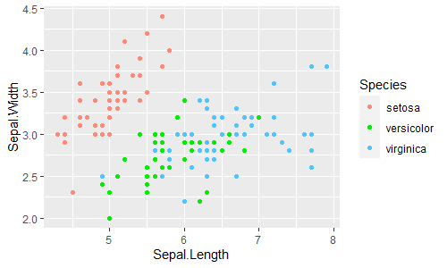
scale_color_discrete(), scale_fill_discrete()：離散値のcolor軸, fill軸

R

ggplot(data = iris, aes(x = Sepal.Length, y = Sepal.Width)) +
  geom_point(aes(color = Species))
ggplot(data = iris, aes(x = Sepal.Length, y = Sepal.Width)) +
  geom_point(aes(color = Species)) +
  scale_color_discrete()
ggplot(data = iris, aes(x = Sepal.Length, y = Sepal.Width)) +
  geom_point(aes(color = Species)) +
  scale_color_discrete(type = getOption("ggplot2.discrete.colour"))

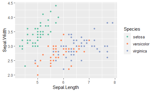
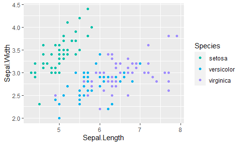
scale_color_viridis_d(), scale_fill_viridis_d()：離散値のcolor軸, fill軸

R

ggplot(data = iris, aes(x = Sepal.Length, y = Sepal.Width)) +
  geom_point(aes(color = Species)) +
  scale_color_viridis_d()
ggplot(data = iris, aes(x = Sepal.Length, y = Sepal.Width)) +
  geom_point(aes(color = Species)) +
  scale_color_viridis_d(alpha = 1, begin = 0, end = 1, direction = 1,
                        option = "D")

scale_shape_*()：shape軸

scale_shape_discrete(), scale_shape_binned()：離散値のshape軸, 連続値のshape軸のビン分割

引数solid：shapeの塗りつぶし

shapeを塗りつぶすかどうかを指定します。デフォルトはsolid = TRUEで塗りつぶします。

R

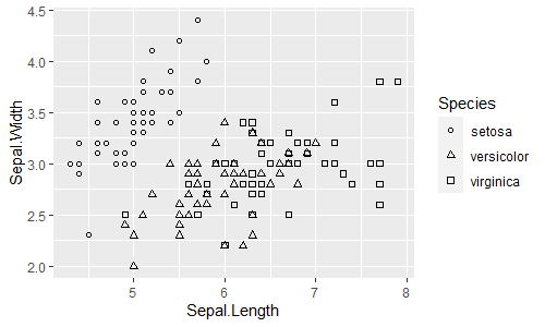
ggplot(data = iris, aes(x = Sepal.Length, y = Sepal.Width)) +
  geom_point(aes(shape = Species)) +
  scale_shape_discrete()
ggplot(data = iris, aes(x = Sepal.Length, y = Sepal.Width)) +
  geom_point(aes(shape = Species)) +
  scale_shape_discrete(solid = TRUE)  # デフォルト

ggplot(data = iris, aes(x = Sepal.Length, y = Sepal.Width)) +
  geom_point(aes(shape = Species)) +
  scale_shape_discrete(solid = FALSE)

R

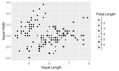
ggplot(data = iris, aes(x = Sepal.Length, y = Sepal.Width)) +
  geom_point(aes(shape = Petal.Length)) +
  scale_shape_binned()  # デフォルト
ggplot(data = iris, aes(x = Sepal.Length, y = Sepal.Width)) +
  geom_point(aes(shape = Petal.Length)) +
  scale_shape_binned(solid = TRUE)

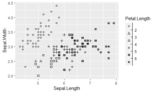
ggplot(data = iris, aes(x = Sepal.Length, y = Sepal.Width)) +
  geom_point(aes(shape = Petal.Length)) +
  scale_shape_binned(solid = FALSE)

まとめ

scale_*()関数を一覧にしておきます。

軸	連続値	連続値のビン分割	離散値	離散値の手動設定	値そのまま
x	scale_x_ continuous()	scale_x_ binned()	scale_x_ discrete()
y	scale_y_ continuous()	scale_y_ binned()	scale_y_ discrete()
color	scale_color_ continuous()	scale_color_ binned()	scale_color_ discrete()	scale_color_ manual()	scale_color_ identity()
colour	scale_colour_ continuous()	scale_colour_ binned()	scale_colour_ discrete()	scale_colour_ manual()	scale_colour_ identity()
fill	scale_fill_ continuous()	scale_fill_ binned()	scale_fill_ discrete()	scale_fill_ manual()	scale_fill_ identity()
alpha	scale_alpha_ continuous()	scale_alpha_ binned()	scale_alpha_ discrete()	scale_alpha_ manual()	scale_alpha_ identity()
size	scale_size_ continuous()	scale_size_ binned()	scale_size_ discrete()	scale_size_ manual()	scale_size_ identity()
shape		scale_shape_ binned()	scale_shape_ discrete()	scale_shape_ manual()	scale_shape_ identity()
linetype		scale_linetype_ binned()	scale_linetype_ discrete()	scale_linetype_ manual()	scale_linetype_ identity()

color軸, colour軸, fill軸にはさらに次の関数もあります。引数も書いておきます。

	連続値	連続値のビン分割	離散値
（再掲）	scale_*_ continuous(type, trans = "reverse", )	scale_*_ binned(type, trans = "reverse", )	scale_*_ discrete(type, trans = "reverse", )
2色のグラデーション (low-high)	scale_*_ gradient(low, high, )	scale_*_ steps(low, high, )
3色のグラデーション (low-mid-high)	scale_*_ gradient2(low, mid, high, midpoint, )	scale_*_ steps2(low, high, mid, midpoint, )
n色のグラデーション	scale_*_ gradientn(colors, )	scale_*_ stepsn(colors, )
グレースケール			scale_*_ grey(start, end, )
色相hue			scale_*_ hue(h, c, l, direction = -1, )
ColorBrewerパレット	scale_*_ distiller(palette, direction = -1, )	scale_*_ fermenter(palette, direction = -1, )	scale_*_ brewer(palette, direction = -1, )
viridisLiteパレット	scale_*_ viridis_c(option, direction = -1, )	scale_*_ viridis_b(option, direction = -1, )	scale_*_ viridis_d(option, direction = -1, )

注）太字は色の反転

参考文献

• https://ggplot2.tidyverse.org/
  • https://ggplot2.tidyverse.org/reference/index.html
• https://github.com/tidyverse/ggplot2
  • https://github.com/rstudio/cheatsheets/blob/master/data-visualization-2.1.pdf
• https://cran.r-project.org/web/packages/ggplot2/index.html
  • https://cran.r-project.org/web/packages/ggplot2/readme/README.html
• https://rstudio.cloud/learn/cheat-sheets
• https://ggplot2-book.org/index.html
  • https://ggplot2-book.org/scales.html
• https://r-graphics.org/
• https://r4ds.had.co.nz/data-visualisation.html
  • https://r4ds.had.co.nz/graphics-for-communication.html
• https://ropensci.github.io/plotly/ggplot2/index.html
• https://heavywatal.github.io/rstats/ggplot2.html
• https://yukiyanai.github.io/jp/classes/stat2/contents/R/intro-to-ggplot2.html
• https://www.jaysong.net/RBook/
  • https://www.jaysong.net/RBook/visualization1.html
  • https://www.jaysong.net/RBook/visualization2.html
  • https://www.jaysong.net/RBook/visualization3.html
  • https://www.jaysong.net/RBook/visualization4.html
• https://kazutan.github.io/fukuokaR11/intro_ggplot2.html
• https://triadsou.hatenablog.com/entry/20100528/1275042816
• https://qiita.com/swathci/items/b36e493ea78b03db0981
• https://qiita.com/swathci/items/b08496d863bca4b479b3

---

1. ggplot2のカラーの綴りは正確にはイギリス式の"colour"ですが、"color"と書いても基本的には動きます（一部例外があります。脚注2.参照。）。以下では"color"で統一します。 ↩

2. ggplot2の"colour"は"color"と書いても基本的には動きますが、scale_color_viridis_b()だけは例外のようです。） ↩