kerasでmixupをやってみた

mixupとは

画像などの入力データを混ぜ合わせてaugmentationする手法として登場したもので、例えばfashion mixupだと以下のようになります。

ラベルはどうするのかというと、画像の混合比率でラベルを算出するわけです。そんなので良いのか？と思うわけですがやらないよりは良い結果が出ることがあるのでkaggleでも盛んにやられているようです。

一方、そんなので良いのか？という考察を進めて、コンテキストが整理された後の方のレイヤー出力を混ぜ合わせてやればもっと上手く機能するだろうというのがmanifold mixupだそうです。
https://arxiv.org/abs/1806.05236

スイスロールデータを使った分かりやすい例が上記論文に出てくるんですが、画像(a)を見ても分かるように入力段でmixupしてしまうと青と青の間に赤がある場所に青を置いてしまうことようなmixupが発生して上手くいかないのがよく分かります。これを後の方のコンテキストが整理されたレイヤー（下画像e）でmixupすれば上手くいきそうだというのが直観的に分かると思います。

やり方

入力データの前処理の場合、処理済みデータを作っておいてから学習する方法もよく用いられますが、mixupの場合はデータ件数の二乗 × 混合比率の場合の数 だけのバリエーションがあるので前処理データを作成しておいて学習するというやり方だとメモリまたはストレージが大量に取られてしまいます。これを避ける為に逐次ランダムにmixupするような書き方として以下のどちらかが良いと思います。

1. tf.dataで前処理的にmixupする
2. カスタムモデルでmixupする

1. tf.dataで前処理的にmixupする

前処理として使う場合はtf.dataで書くのがやりやすいと思います
この場合manifold mixupは出来ませんが、他の前処理と組み合わせて書くのに適しています

作例がkeras.ioにあったのでこれをやっていきたいと思います
https://keras.io/examples/vision/mixup/

tf.dataの使い方が分からない人は以下
https://qiita.com/studio_haneya/items/1138e427367e93cd2ab8

1-1. 準備

fashion mnistのデータを使っていきます

import numpy as np
import tensorflow as tf
import matplotlib.pyplot as plt
from tensorflow.keras import layers

(x_train, y_train), (x_test, y_test) = tf.keras.datasets.fashion_mnist.load_data()

x_train = x_train.astype("float32") / 255.0
x_train = np.reshape(x_train, (-1, 28, 28, 1))
y_train = tf.one_hot(y_train, 10)

x_test = x_test.astype("float32") / 255.0
x_test = np.reshape(x_test, (-1, 28, 28, 1))
y_test = tf.one_hot(y_test, 10)

plt.imshow(x_train[0])
plt.show()

1-2. mixupする

バッチサイズや学習回数を指定しておきます

AUTO = tf.data.AUTOTUNE
BATCH_SIZE = 64
EPOCHS = 10

shuffleしてバッチサイズ64で取り出すtf.data.Dataset2つをつくります

# Put aside a few samples to create our validation set
val_samples = 2000
x_val, y_val = x_train[:val_samples], y_train[:val_samples]
new_x_train, new_y_train = x_train[val_samples:], y_train[val_samples:]

train_ds_one = (
    tf.data.Dataset.from_tensor_slices((new_x_train, new_y_train))
    .shuffle(BATCH_SIZE * 100)
    .batch(BATCH_SIZE)
)
train_ds_two = (
    tf.data.Dataset.from_tensor_slices((new_x_train, new_y_train))
    .shuffle(BATCH_SIZE * 100)
    .batch(BATCH_SIZE)
)
# Because we will be mixing up the images and their corresponding labels, we will be
# combining two shuffled datasets from the same training data.
train_ds = tf.data.Dataset.zip((train_ds_one, train_ds_two))
val_ds = tf.data.Dataset.from_tensor_slices((x_val, y_val)).batch(BATCH_SIZE)
test_ds = tf.data.Dataset.from_tensor_slices((x_test, y_test)).batch(BATCH_SIZE)

mixupする処理を追加します
この作例ではガンマ分布で混合比率をつくっていますね

def sample_beta_distribution(size, concentration_0=0.2, concentration_1=0.2):
    gamma_1_sample = tf.random.gamma(shape=[size], alpha=concentration_1)
    gamma_2_sample = tf.random.gamma(shape=[size], alpha=concentration_0)
    return gamma_1_sample / (gamma_1_sample + gamma_2_sample)


def mix_up(ds_one, ds_two, alpha=0.2):
    # Unpack two datasets
    images_one, labels_one = ds_one
    images_two, labels_two = ds_two
    batch_size = tf.shape(images_one)[0]

    # Sample lambda and reshape it to do the mixup
    l = sample_beta_distribution(batch_size, alpha, alpha)
    x_l = tf.reshape(l, (batch_size, 1, 1, 1))
    y_l = tf.reshape(l, (batch_size, 1))

    # Perform mixup on both images and labels by combining a pair of images/labels
    # (one from each dataset) into one image/label
    images = images_one * x_l + images_two * (1 - x_l)
    labels = labels_one * y_l + labels_two * (1 - y_l)
    return (images, labels)

# First create the new dataset using our `mix_up` utility
train_ds_mu = train_ds.map(
    lambda ds_one, ds_two: mix_up(ds_one, ds_two, alpha=0.2), num_parallel_calls=AUTO
)

どうなってるか確認します

# Let's preview 9 samples from the dataset
sample_images, sample_labels = next(iter(train_ds_mu))
plt.figure(figsize=(10, 10))
for i, (image, label) in enumerate(zip(sample_images[:9], sample_labels[:9])):
    ax = plt.subplot(3, 3, i + 1)
    plt.imshow(image.numpy().squeeze())
    print(label.numpy().tolist())
    plt.axis("off")

混合比率のヒストグラムをとるとこんな感じになっています

どちらかに近いものが多めに生成されて中間的なものは少なめという設定にしているようです

1-3. 学習する

def get_training_model():
    model = tf.keras.Sequential(
        [
            layers.Conv2D(16, (5, 5), activation="relu", input_shape=(28, 28, 1)),
            layers.MaxPooling2D(pool_size=(2, 2)),
            layers.Conv2D(32, (5, 5), activation="relu"),
            layers.MaxPooling2D(pool_size=(2, 2)),
            layers.Dropout(0.2),
            layers.GlobalAvgPool2D(),
            layers.Dense(128, activation="relu"),
            layers.Dense(10, activation="softmax"),
        ]
    )
    return model

model = get_training_model()
model.load_weights("initial_weights.h5")
model.compile(loss="categorical_crossentropy", optimizer="adam", metrics=["accuracy"])
model.fit(train_ds_mu, validation_data=val_ds, epochs=EPOCHS)
_, test_acc = model.evaluate(test_ds)
print("Test accuracy: {:.2f}%".format(test_acc * 100))

Epoch 1/10
907/907 [==============================] - 7s 5ms/step - loss: 1.1765 - accuracy: 0.6317 - val_loss: 0.6789 - val_accuracy: 0.7530
Epoch 2/10
907/907 [==============================] - 7s 8ms/step - loss: 0.9215 - accuracy: 0.7360 - val_loss: 0.5491 - val_accuracy: 0.8100
Epoch 3/10
907/907 [==============================] - 6s 6ms/step - loss: 0.8400 - accuracy: 0.7738 - val_loss: 0.4659 - val_accuracy: 0.8465
Epoch 4/10
907/907 [==============================] - 5s 6ms/step - loss: 0.7875 - accuracy: 0.7929 - val_loss: 0.4409 - val_accuracy: 0.8530
Epoch 5/10
907/907 [==============================] - 6s 6ms/step - loss: 0.7553 - accuracy: 0.8037 - val_loss: 0.4107 - val_accuracy: 0.8575
Epoch 6/10
907/907 [==============================] - 6s 6ms/step - loss: 0.7327 - accuracy: 0.8091 - val_loss: 0.3795 - val_accuracy: 0.8715
Epoch 7/10
907/907 [==============================] - 5s 6ms/step - loss: 0.7016 - accuracy: 0.8190 - val_loss: 0.3798 - val_accuracy: 0.8705
Epoch 8/10
907/907 [==============================] - 7s 7ms/step - loss: 0.6906 - accuracy: 0.8216 - val_loss: 0.3545 - val_accuracy: 0.8740
Epoch 9/10
907/907 [==============================] - 5s 6ms/step - loss: 0.6817 - accuracy: 0.8264 - val_loss: 0.3454 - val_accuracy: 0.8805
Epoch 10/10
907/907 [==============================] - 5s 6ms/step - loss: 0.6691 - accuracy: 0.8299 - val_loss: 0.3665 - val_accuracy: 0.8670
157/157 [==============================] - 1s 3ms/step - loss: 0.3934 - accuracy: 0.8618
Test accuracy: 86.18%

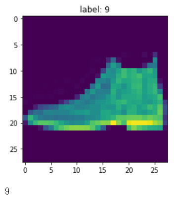
1-4. 推定例

k = 0
x, y = next(iter(test_ds))
plt.imshow(x[k])
plt.title('label: {}'.format(np.where(y[k])[0][0]))
plt.show()

y_pred = model.predict(x)
np.argmax(y_pred[k])

2. カスタムモデルでmixupする

shuffleのみtf.dataでやって、mixupをカスタムモデル内で実行するやり方です。manifold mixupするときはこちらでやる事になると思います。そのままh5ファイルで書き出すことが出来なくなるし、デバッグがやりにくいのが面倒ですが、manifold mixupする場合はこれしかないかなと思います。

カスタムモデルの作り方は先日書いたのでそちらを参照してください
https://qiita.com/studio_haneya/items/fc89b20f51e2feb90ab3

2-1. 準備

データの準備は上と重複してますが一応書いておきます

データの読み込み

import numpy as np
import tensorflow as tf
import matplotlib.pyplot as plt

def load_fashion_mnist_data(digits=False):
    (x_train, y_train), (x_test, y_test) = tf.keras.datasets.fashion_mnist.load_data()

    x_train = x_train.astype("float32") / 255.0
    x_train = np.reshape(x_train, (-1, 28, 28, 1))
    if digits:
        y_train = tf.one_hot(y_train, 10)

    x_test = x_test.astype("float32") / 255.0
    x_test = np.reshape(x_test, (-1, 28, 28, 1))
    if digits:
        y_test = tf.one_hot(y_test, 10)

    x_val, y_val = x_train[:val_samples], y_train[:val_samples]
    x_train, y_train = x_train[val_samples:], y_train[val_samples:]

    print(x_train.shape, y_train.shape)
    print(x_val.shape, y_val.shape)
    print(x_test.shape, y_test.shape)

    k = 2
    plt.imshow(x_train[k])
    plt.title(y_train[k])
    plt.show()

    return x_train, y_train, x_val, y_val, x_test, y_test

x_train, y_train, x_val, y_val, x_test, y_test = load_fashion_mnist_data()

学習データのみ入力が2つあって

tf.data.Datasetの作成

# Put aside a few samples to create our validation set
val_samples = 2000
x_val, y_val = x_train[:val_samples], y_train[:val_samples]
new_x_train, new_y_train = x_train[val_samples:], y_train[val_samples:]

train_ds_one = (
    tf.data.Dataset.from_tensor_slices((new_x_train, new_y_train))
    .shuffle(BATCH_SIZE * 100)
    .batch(BATCH_SIZE)
)
train_ds_two = (
    tf.data.Dataset.from_tensor_slices((new_x_train, new_y_train))
    .shuffle(BATCH_SIZE * 100)
    .batch(BATCH_SIZE)
)
# Because we will be mixing up the images and their corresponding labels, we will be
# combining two shuffled datasets from the same training data.
train_ds = tf.data.Dataset.zip((train_ds_one, train_ds_two))
val_ds = tf.data.Dataset.from_tensor_slices((x_val, y_val)).batch(BATCH_SIZE)
test_ds = tf.data.Dataset.from_tensor_slices((x_test, y_test)).batch(BATCH_SIZE)

2-2. 中身のモデルをつくる

mixupの前に通すモデルと、mixupの後に通すモデルを作ります

def make_before_mixup_model():
    inputs = tf.keras.layers.Input(shape=(28, 28, 1))    
    network = tf.keras.layers.Conv2D(16, (3, 3), strides=(2, 2), padding="same")(inputs)
    network = tf.keras.layers.LeakyReLU(alpha=0.2)(network)
    network = tf.keras.layers.MaxPooling2D(pool_size=(2, 2), strides=(1, 1), padding="same")(network)
    network = tf.keras.layers.Conv2D(32, (3, 3), strides=(2, 2), padding="same")(network)
    outputs = tf.keras.layers.Flatten()(network)
    model = tf.keras.models.Model(inputs, outputs)
    return model

def make_after_mixup_model(input_shape):
    inputs = tf.keras.layers.Input(shape=(input_shape))
    outputs = tf.keras.layers.Dense(10)(inputs)
    model = tf.keras.models.Model(inputs, outputs)
    return model

before_mixup = make_before_mixup_model()
after_mixup = make_after_mixup_model(before_mixup.output_shape[1:])

2-3. カスタムモデルをつくる

最初にやったのと同様にベータ分布で混合比をつくって、x側とy側を同じ比率でmixupします。混合比はバッチごとに毎回変えたいのでtrain_step()内で作成するようにしています。

学習時は入力を(x1, x2), (y1, y2)と2つずつ受け取ってmixupしながら学習しますが、推定時は不要なのでx, yを1つずつ受け取るだけになります。

class MixupModel(tf.keras.Model):
    def __init__(self, before_mixup, after_mixup, **kwargs):
        super(MixupModel, self).__init__(**kwargs)
        self.before_mixup = before_mixup
        self.after_mixup = after_mixup

    def compile(self, optimizer, metrics, alpha=0.2, **kwargs):
        super(MixupModel, self).compile(optimizer=optimizer, metrics=metrics, **kwargs)
        self.alpha = alpha

    def sample_beta_distribution(self, size):
        gamma_1_sample = tf.random.gamma(shape=[size], alpha=self.alpha)
        gamma_2_sample = tf.random.gamma(shape=[size], alpha=self.alpha)
        return gamma_1_sample / (gamma_1_sample + gamma_2_sample)

    @staticmethod
    def mixup(x1, x2, alpha_tensor):
        size = x1.shape[0]
        count = tf.reduce_prod(x1.shape[1:])

        for _ in range(len(x1.shape) - 1):
            alpha_tensor = tf.expand_dims(alpha_tensor, -1)

        return x1 * alpha_tensor + x2 * (1 - alpha_tensor)

    def call(self, inputs, training=False):
        t = self.before_mixup(inputs, training=training)
        y_pred = self.after_mixup(t, training=training)
        return y_pred

    def train_step(self, data):
        x, y, sample_weight = tf.keras.utils.unpack_x_y_sample_weight(data)
        x1, x2 = x
        y1, y2 = y

        alpha_tensor = self.sample_beta_distribution(tf.shape(x1)[0])
        y = self.mixup(y1, y2, alpha_tensor)

        with tf.GradientTape() as tape:
            t1 = self.before_mixup(x1, training=True)
            t2 = self.before_mixup(x2, training=True)
            t = self.mixup(t1, t2, alpha_tensor)
            y_pred = self.after_mixup(t)
            loss = self.compiled_loss(y, y_pred)

        gradients = tape.gradient(loss, self.trainable_variables)
        self.optimizer.apply_gradients(zip(gradients, self.trainable_variables))
        self.compiled_metrics.update_state(y, y_pred, sample_weight)
        return {m.name: m.result() for m in self.metrics}

    def test_step(self, data):
        x, y, sample_weight = tf.keras.utils.unpack_x_y_sample_weight(data)
        y_pred = self(x, training=True)
        loss = self.compiled_loss(y, y_pred)
        self.compiled_metrics.update_state(y, y_pred, sample_weight)
        return {m.name: m.result() for m in self.metrics}

2-4. 学習する

model = MixupModel(before_mixup, after_mixup)

loss = tf.keras.losses.CategoricalCrossentropy(from_logits=True)
model.compile(loss=loss, optimizer="adam", metrics=["accuracy"])

model.fit(train_ds, validation_data=val_ds, epochs=5)
print(model.evaluate(x_test, y_test))

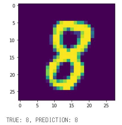
y_pred = model(x_test)

k = np.random.randint(0, x_test.shape[0], 1)[0]
plt.imshow(x_test[k])
plt.show()
print('TRUE: {}, PREDICTION: {}'.format(np.argmax(y_test[k]), np.argmax(y_pred[k])))

Epoch 1/5
907/907 [==============================] - 7s 7ms/step - loss: 0.6292 - accuracy: 0.8881 - val_loss: 0.1641 - val_accuracy: 0.9610
Epoch 2/5
907/907 [==============================] - 7s 7ms/step - loss: 0.4656 - accuracy: 0.9441 - val_loss: 0.1335 - val_accuracy: 0.9705
Epoch 3/5
907/907 [==============================] - 6s 6ms/step - loss: 0.4416 - accuracy: 0.9514 - val_loss: 0.1223 - val_accuracy: 0.9725
Epoch 4/5
907/907 [==============================] - 6s 6ms/step - loss: 0.4361 - accuracy: 0.9536 - val_loss: 0.1185 - val_accuracy: 0.9750
Epoch 5/5
907/907 [==============================] - 6s 6ms/step - loss: 0.4322 - accuracy: 0.9567 - val_loss: 0.1178 - val_accuracy: 0.9810
313/313 [==============================] - 1s 3ms/step - loss: 0.1085 - accuracy: 0.9783
[0.10854344815015793, 0.9782999753952026]

まとめ

manifold mixupについてもウェブ上に実装例がいくつか見つかるんですが、書き方がかなり独特だったので普通のカスタムモデルで書いてみました。こちらのお作法に慣れている方には読みやすくできたんじゃないかと思います。レッツトライ