opencv-python画像処理入門

機械学習用の画像の前処理方法を調べたのを書いていきます。
中途半端な内容ですが、今後書き足していくと思います。

試行環境

Windows10
python 3.6
opencv-python 4.1.2.30

閾値処理: cv.Threshold(src, threshold, maxValue, thresholdType)

opencvドキュメント
http://labs.eecs.tottori-u.ac.jp/sd/Member/oyamada/OpenCV/html/py_tutorials/py_imgproc/py_thresholding/py_thresholding.html

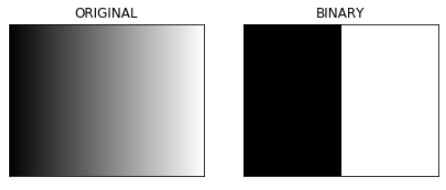
閾値を指定して二値化

適当なグラデーション画像を作って二値化してみます

# make gray scale picture
im_gray = np.array([np.arange(0, 256, 2) for k in range(100)])
im_gray = im_gray.astype('uint8')
print(im_gray.shape)

# apply threshold
ret, thresh1 = cv2.threshold(im_gray,127,255,cv2.THRESH_BINARY)

# show picture
plt.figure(figsize=(7, 6))

ax = plt.subplot(1, 2, 1)
ax.imshow(im_gray, 'gray')
ax.set_xticks([])
ax.set_yticks([])
ax.set_title('ORIGINAL')

ax = plt.subplot(1, 2, 2)
ax.imshow(thresh1, 'gray')
ax.set_xticks([])
ax.set_yticks([])
ax.set_title('BINARY')

plt.show()

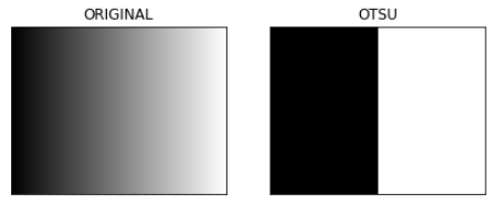
閾値を自動で設定して二値化

大津の方法を使って2値化します

# make gray scale picture
im_gray = np.array([np.arange(0, 256, 2) for k in range(100)])
im_gray = im_gray.astype('uint8')
print(im_gray.shape)

# global thresholding
ret1,th1 = cv2.threshold(im_gray,127,255,cv2.THRESH_BINARY)

# Otsu's thresholding
ret2,th2 = cv2.threshold(im_gray,0,255,cv2.THRESH_BINARY+cv2.THRESH_OTSU)


# show picture
plt.figure(figsize=(7, 6))

ax = plt.subplot(1, 2, 1)
ax.imshow(im_gray, 'gray')
ax.set_xticks([])
ax.set_yticks([])
ax.set_title('ORIGINAL')

ax = plt.subplot(1, 2, 2)
ax.imshow(thresh1, 'gray')
ax.set_xticks([])
ax.set_yticks([])
ax.set_title('OTSU')

plt.show()

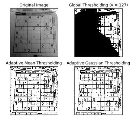
動的な閾値で二値化: adaptiveThreshold(src, maxValue, adaptiveMethod, thresholdType, blockSize, C[, dst])

写真画像など明度のグラデーションがあって１つの閾値で画像全体を二値化できない場合に使います

http://labs.eecs.tottori-u.ac.jp/sd/Member/oyamada/OpenCV/html/py_tutorials/py_imgproc/py_thresholding/py_thresholding.html

import cv2
import numpy as np
from matplotlib import pyplot as plt

img = cv2.imread('../input/dave.jpg',0)
img = cv2.medianBlur(img,5)

ret,th1 = cv2.threshold(img,127,255,cv2.THRESH_BINARY)
th2 = cv2.adaptiveThreshold(img,255,cv2.ADAPTIVE_THRESH_MEAN_C,\
            cv2.THRESH_BINARY,11,2)
th3 = cv2.adaptiveThreshold(img,255,cv2.ADAPTIVE_THRESH_GAUSSIAN_C,\
            cv2.THRESH_BINARY,11,2)

titles = ['Original Image', 'Global Thresholding (v = 127)',
            'Adaptive Mean Thresholding', 'Adaptive Gaussian Thresholding']
images = [img, th1, th2, th3]

plt.figure(figsize=(6.5, 6))
for i in range(4):
    plt.subplot(2,2,i+1),plt.imshow(images[i],'gray')
    plt.title(titles[i])
    plt.xticks([]),plt.yticks([])
plt.show()

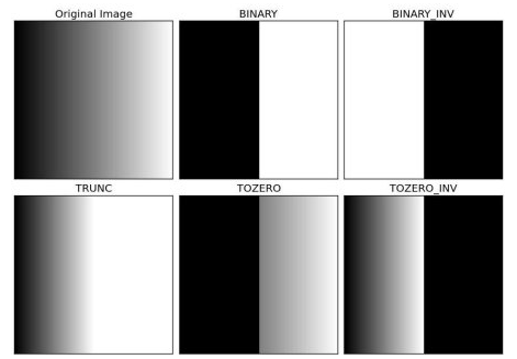
その他の閾値処理

よく使う二値化以外にもthresholdTypeにはいろいろあります

# make gray scale picture
im_gray = np.array([np.arange(0, 256, 2) for k in range(100)])
im_gray = im_gray.astype('uint8')
print(im_gray.shape)

# apply threshold
ret,thresh1 = cv2.threshold(im_gray,127,255,cv2.THRESH_BINARY)
ret,thresh2 = cv2.threshold(im_gray,127,255,cv2.THRESH_BINARY_INV)
ret,thresh3 = cv2.threshold(im_gray,127,255,cv2.THRESH_TRUNC)
ret,thresh4 = cv2.threshold(im_gray,127,255,cv2.THRESH_TOZERO)
ret,thresh5 = cv2.threshold(im_gray,127,255,cv2.THRESH_TOZERO_INV)

# show result
titles = ['Original Image','BINARY','BINARY_INV','TRUNC','TOZERO','TOZERO_INV']
images = [im_gray, thresh1, thresh2, thresh3, thresh4, thresh5]

for i in range(6):
    plt.subplot(2,3,i+1)
    plt.imshow(images[i],'gray')
    plt.title(titles[i])
    plt.xticks([]),plt.yticks([])
plt.show()

画像の読み込み: cv2.imread()

ここからは適当な画像ファイルを読み込んで使っていきます。cv2.imread()するとnumpy.arrayとして画像を読み込めます。画像の表示はcv2.imshow()かplt.imshow()を使いますが、cv2.imshow()はjupyter notebookで動かないようなので、plt.imshow()で表示していきます。ただし、opencvは伝統的にBGRで値を読んでくる一方で、plt.imshow()はRGBであるとして表示しますので、cv2.cvtColor(src, cv2.COLOR_BGR2RGB)でRとBを入れ替えてから表示してやります。

python

import cv2
import matplotlib.pyplot as plt

im = cv2.imread('../input/opencv.png')

plt.imshow(cv2.cvtColor(im, cv2.COLOR_BGR2RGB))
plt.xticks([])
plt.yticks([])
plt.show()

今回はこの画像でやっていきます

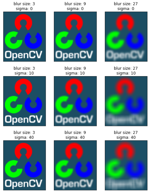
画像をぼかす: cv2.GaussianBlur(src, (size, size), sigma)

opencvドキュメント
http://labs.eecs.tottori-u.ac.jp/sd/Member/oyamada/OpenCV/html/py_tutorials/py_imgproc/py_filtering/py_filtering.html

画像をぼかすフィルターです。
sizeが縦横サイズ、sigmaが縦横の標準偏差です。sigmaも縦横それぞれ指定することが出来ますが、省略すると縦横とも同じ標準偏差を使用します。size、sigmaとも大きくするとボケる度合が強くなります。

python

plt.figure(figsize=(8, 10.4))

for k, size in enumerate([3, 9, 27]):
    for k2, sigma in enumerate([0, 10, 40]):
        blur = cv2.GaussianBlur(im, (size, size), sigma)
        ax = plt.subplot(3, 3, k2*3+k+1)
        ax.imshow(cv2.cvtColor(blur, cv2.COLOR_BGR2RGB))
        ax.set_xticks([])
        ax.set_yticks([])
        ax.set_title('blur size: %d\nsigma: %d' % (size, sigma))
plt.show()

アルファ合成: addWeighted(src1, alpha, src2, beta, gamma)

opencvドキュメント
https://docs.opencv.org/2.4/modules/core/doc/operations_on_arrays.html

こんな感じで混ぜ合わせた画像が作れます。また、alpha, betaに1より大きい値を入れる事ができますが値が大きい画素は値が振り切るので右端の画像のようにちょっと不思議な混じり方をします。

python

im2 = cv2.imread('../input/black_white.png')[:,:,::-1]
plt.imshow(cv2.cvtColor(im2, cv2.COLOR_BGR2RGB))

python

plt.figure(figsize=(15, 20))
for k, alpha in enumerate([0, 0.25, 0.5, 0.75, 1]):
    for k2, gamma in enumerate([0, 0.5, 1, 2, 4]):
        beta = 1 - alpha
        im3 = cv2.addWeighted(im, alpha, im2, beta, gamma)

        ax = plt.subplot(5, 5, 5*k2+k+1)
        ax.imshow(cv2.cvtColor(im3, cv2.COLOR_BGR2RGB))
        ax.set_title('alpha: %1.2f\nbeta: %1.2f\ngamma: %1.2f' % (alpha, beta, gamma))
        ax.set_xticks([])
        ax.set_yticks([])
plt.show()

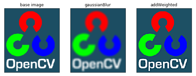
ぼかしとアルファ合成を使って輪郭強調

ぼかした画像を元画像から引くようにすると輪郭を強調できます。

python

blur = cv2.GaussianBlur(im, (9, 9), 27)
im3 = cv2.addWeighted(im, 1.5, blur, -0.5, 1)

plt.figure(figsize=(10, 5))

ax = plt.subplot(1, 3, 1)
ax.imshow(cv2.cvtColor(im, cv2.COLOR_BGR2RGB))
ax.set_title('base image')
ax.set_xticks([])
ax.set_yticks([])

ax = plt.subplot(1, 3, 2)
ax.imshow(cv2.cvtColor(blur, cv2.COLOR_BGR2RGB))
ax.set_title('gaussianBlur')
ax.set_xticks([])
ax.set_yticks([])

ax = plt.subplot(1, 3, 3)
ax.imshow(cv2.cvtColor(im3, cv2.COLOR_BGR2RGB))
ax.set_title('addWeighted')
ax.set_xticks([])
ax.set_yticks([])

plt.show()

元の画像をalpha=1.5、ブラーをかけた画像をbeta=-0.5で混合すると輪郭が強調された画像になります。

フィルタ処理: cv2.filter2D(src, kernel)

畳み込みフィルタ関数です。配列の値を変えるといろんなフィルタ処理を実装できるようです。上でやっていたgaussianBlur()もこの関数で実装できます。

平行移動

kernelを[1]にすると元の画像と同じものが出来ます。
また、それなりに大きい配列のどこかを1、他は全部0にすると以下のように平行移動させることもできます。

python

size = 21
kernel = np.zeros(size**2).reshape(size, size)
kernel[0, 0] = 1
kernel = kernel / np.sum(kernel)
print(kernel)

im4 = cv2.filter2D(im, -1, kernel)


# show picture
plt.figure(figsize=(7, 6))

ax = plt.subplot(1, 2, 1)
ax.imshow(cv2.cvtColor(im, cv2.COLOR_BGR2RGB))
ax.set_xticks([])
ax.set_yticks([])
ax.set_title('base image')

ax = plt.subplot(1, 2, 2)
ax.imshow(cv2.cvtColor(im4, cv2.COLOR_BGR2RGB))
ax.set_xticks([])
ax.set_yticks([])
ax.set_title('moved')

plt.show()

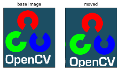
足りない分は鏡像が反転して出てきます。

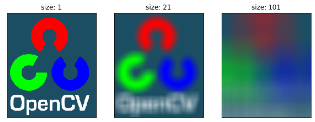
平均フィルタ

kernelを全部同じ値、合計１になるようにすると平均フィルタになります。
cv2.blur()と同じです。

python

def average_filter(size, im):
    kernel = np.ones(size**2).reshape(size, size)
    kernel = kernel / np.sum(kernel)
    im4 = cv2.filter2D(im, -1, kernel)
    return im4

plt.figure(figsize=(10, 5))
for k, size in enumerate([1, 21, 101]):
    im4 = average_filter(size, im)
    ax = plt.subplot(1, 3, k+1)

    ax.imshow(cv2.cvtColor(im4, cv2.COLOR_BGR2RGB))
    ax.set_title('size: %d' % size)
    ax.set_xticks([])
    ax.set_yticks([])
plt.show()

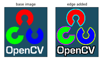
輪郭強調フィルタ

以下のように合計1、中央以外を全部マイナス1にすると輪郭強調フィルタになります。

\begin{pmatrix}
-1 & -1 & -1 & -1 & -1 & -1 & -1 \\
-1 & -1 & -1 & -1 & -1 & -1 & -1 \\
-1 & -1 & -1 & -1 & -1 & -1 & -1 \\
-1 & -1 & -1 & 49 & -1 & -1 & -1 \\
-1 & -1 & -1 & -1 & -1 & -1 & -1 \\
-1 & -1 & -1 & -1 & -1 & -1 & -1 \\
-1 & -1 & -1 & -1 & -1 & -1 & -1
\end{pmatrix}

python

def edge_filter(size, im):
    kernel = np.full(size**2, -1).reshape(size, size)
    pos = int((size-1)/2)
    kernel[pos, pos] = size**2
    print(kernel)
    im4 = cv2.filter2D(im, -1, kernel)
    return im4

im4 = edge_filter(7, im)

plt.figure(figsize=(6, 5))

ax = plt.subplot(1, 2, 1)
ax.imshow(cv2.cvtColor(im, cv2.COLOR_BGR2RGB))
ax.set_title('base image')
ax.set_xticks([])
ax.set_yticks([])

ax = plt.subplot(1, 2, 2)
ax.imshow(cv2.cvtColor(im4, cv2.COLOR_BGR2RGB))
ax.set_title('edge added')
ax.set_xticks([])
ax.set_yticks([])

plt.show()

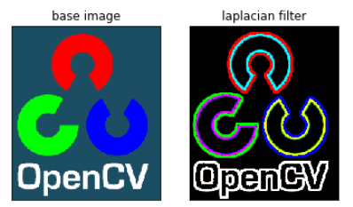
輪郭抽出フィルタ

上のフィルタと似ていますが合計がゼロになるようにしてやると輪郭のみを抽出するようなフィルタになります。

python

def laplacian_filter(size, im):
    kernel = np.ones(size**2).reshape(size, size)
    pos = int((size-1)/2)
    kernel[pos, pos] = -(size**2-1)
    print(kernel)
    im4 = cv2.filter2D(im, -1, kernel)
    return im4

im4 = laplacian_filter(7, im)

plt.figure(figsize=(6, 5))

ax = plt.subplot(1, 2, 1)
ax.imshow(cv2.cvtColor(im, cv2.COLOR_BGR2RGB))
ax.set_title('base image')
ax.set_xticks([])
ax.set_yticks([])

ax = plt.subplot(1, 2, 2)
ax.imshow(cv2.cvtColor(im4, cv2.COLOR_BGR2RGB))
ax.set_title('laplacian filter')
ax.set_xticks([])
ax.set_yticks([])

plt.show()

(追記予定)