目次
以下のこれら記事はPyTorchを使って時系列データの予測をしたい方に向けて書きました.
理論は本や論文をじっくり読む方が良いかと思いましたので,特に実装方法について詳しく書きました.
使用するプログラムの一部は各記事の中で重複しているものもあり,重複した部分を毎回1から説明すると記事が長くなり読みにくいと思うので省略しています.
そのため以下の順番で読み進めていただけると読みやすいかと思います.
- [PyTorch 1.9.0] LSTMを使って時系列(単純な数式)予測してみた<- 現在読んでいただいている記事
- [PyTorch 1.9.0] LSTMを使っていくつ先の未来まで精度良く予測できるのか検証してみた
0. はじめに
初めてLSTMの実装をしていく中で苦労した点をまとめてみました.
LSTMがどういう仕組みで予測を行っているかというところは,本を読む方が良いと思いますので,私はLSTMの実装方法を中心に書きました.
特に私はデータセットの作り方やLSTMに入力するデータの形をどうするかというところに苦労したので,各処理で扱っている配列の形と中身をしっかりと書くことでデータの流れを分かりやすくなるように意識しました.
コードの説明は,基本的にコードのブロックの上で説明するようにしています.したがって説明が見たいコードのブロックがあったらその上の文章を読んでいただければ良いと思います.
事前知識
全てのコード1行ずつ説明するのは中々困難ですので,以下の知識があることを前提に書かせていただきました.
- PyTorchの基礎的な書き方
-
torch.Tensor().to()の使い方 -
train(),eval()で学習と推論のモードを切り替えること(このプログラムではdropoutやbatch normalizationを使っていないのであまり関係はないと思うのですがとりあえず書いとくものではあったりします.) - 学習時には
criterion,optimizer.zero_grad(),loss.backward(),optimizer.step()などの関数を使うこと -
data.cpu().numpy()でネットワークの出力をnumpyに変換すること等...
-
- pythonの基礎的な書き方
- listからnumpyに変換する方法
- Classの書き方
- sklearnの
shuffleやtrain_test_splitの使い方 - matplotの使い方等...
- githubの基礎知識
- git cloneでリポジトリをクローン(ダウンロード)できること等...
問題設定
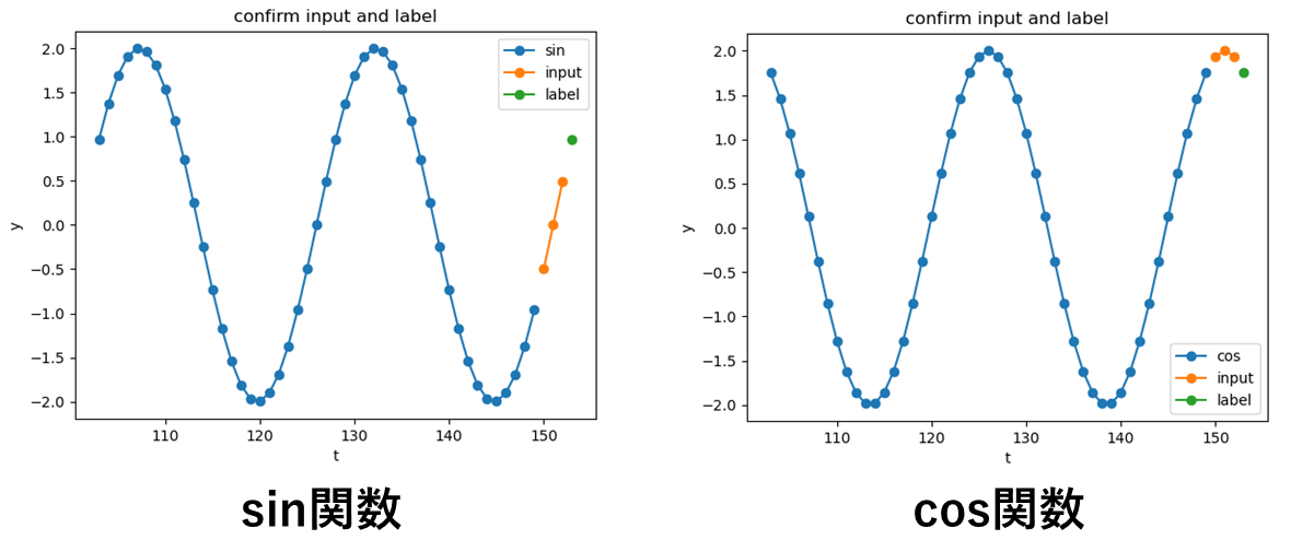
sin関数やcos関数のような単純な数式を使って時系列データを生成し,その数式のいくつかの出力を用いて1つ先の未来の値を予測する問題を設定しました.
イメージとしては以下の図の通りです.
オレンジ色の点から緑の点を求める問題を設定しました.
1. 開発環境
- Ubuntu 18.04
- anaconda 4.10.3
- python 3.8.11
- pytorch 1.9.0
- cudatoolkit 11.1
anacondaを使用している人は,githubにanacondaの環境ファイル(predict_simple_formula_env.yml)を置いているので,そのファイルを使って仮想環境をコピーしていただくとすぐにここで説明しているプログラムを動かせると思います.
anacondaの仮想環境をコピーする方法
以下のコマンドをターミナル上で打つとanacondaの環境ファイルとこの記事で紹介するプログラムを含むリポジトリをダウンロードできます.
git clone https://github.com/sloth-hobby/PyTorch_practice.git
ターミナル上でPyTorch_practice/lstm_practice/envs/のディレクトリ下に移動し,anacondaの仮想環境に入っている状態で以下のコマンドを打つと仮想環境をコピーできます.環境名のところはどんな名前でも良いです.
conda env create -n 環境名 -f predict_simple_formula_env.yml
2. 全体のプログラムの構成
予測のために以下の3つのクラスで機能を分割しました.
各章でクラス内の実装を順番に説明しています.
- 時系列データを作るための単純な数式を定義するクラス.
- ネットワークの構造を定義するクラス.
- 学習用のクラス
この記事で説明するコードの全体(折りたたんでいるのでこれをクリックして頂けると全体が見られます)
import torch
import torch.nn as nn
import torch.nn.functional as F
import torch.optim as optim

from sklearn.model_selection import train_test_split
from sklearn.utils import shuffle
import numpy as np
import matplotlib.pyplot as plt

class SimpleFormula():
    def __init__(self, sin_a=2.0, cos_a = 2.0, sin_t=25.0, cos_t = 25.0):
        self.sin_a = sin_a
        self.cos_a = cos_a
        self.sin_t = sin_t
        self.cos_t = cos_t

    def sin(self, input):
        return self.sin_a * np.sin(2.0 * np.pi / self.sin_t * (input))

    def cos(self, input):
        return self.cos_a * np.cos(2.0 * np.pi / self.cos_t * (input))

class PredictSimpleFormulaNet(nn.Module):
    def __init__(self, input_size, output_size, hidden_size, batch_first):
        super(PredictSimpleFormulaNet, self).__init__()
        self.rnn = nn.LSTM(input_size = input_size,
                            hidden_size = hidden_size,
                            batch_first = batch_first)
        self.output_layer = nn.Linear(hidden_size, output_size)

        nn.init.xavier_normal_(self.rnn.weight_ih_l0)
        nn.init.orthogonal_(self.rnn.weight_hh_l0)

    def forward(self, inputs):
        h, _= self.rnn(inputs)
        output = self.output_layer(h[:, -1])

        return output

class Train():
    def __init__(self, input_size, output_size, hidden_size, batch_first, lr):
        self.device = torch.device('cuda' if torch.cuda.is_available() else 'cpu')
        print("device:", self.device)
        self.net = PredictSimpleFormulaNet(input_size, output_size, hidden_size, batch_first).to(self.device)
        self.criterion = nn.MSELoss(reduction='mean')
        self.optimizer = optim.Adam(self.net.parameters(), lr=lr, betas=(0.9, 0.999), amsgrad=True)

    def set_formula_const_arg(self, sin_a, cos_a, sin_t, cos_t):
        self.f = SimpleFormula(sin_a, cos_a, sin_t, cos_t)

    def make_dataset(self, dataset_num, sequence_length, t_start, calc_mode="sin"):
        dataset_inputs = []
        dataset_labels = []
        dataset_times = []
        for t in range(dataset_num):
            if calc_mode == "sin":
                dataset_inputs.append([self.f.sin(t_start + t + i) for i in range(sequence_length)])
                dataset_labels.append([self.f.sin(t_start + t + sequence_length)])
            elif calc_mode == "cos":
                dataset_inputs.append([self.f.cos(t_start + t + i) for i in range(sequence_length)])
                dataset_labels.append([self.f.cos(t_start + t + sequence_length)])
            dataset_times.append(t_start + t + sequence_length)
        print("test = {}, {}, {}".format(np.array(dataset_inputs).shape,  np.array(dataset_labels).shape, np.array(dataset_times).shape))
        return np.array(dataset_inputs),  np.array(dataset_labels), np.array(dataset_times)

    def train_step(self, inputs, labels):
        inputs = torch.Tensor(inputs).to(self.device)
        labels = torch.Tensor(labels).to(self.device)
        self.net.train()
        preds = self.net(inputs)
        loss = self.criterion(preds, labels)
        self.optimizer.zero_grad()
        loss.backward()
        # 勾配が大きくなりすぎると計算が不安定になるので、clipで最大でも勾配2.0に留める
        nn.utils.clip_grad_value_(self.net.parameters(), clip_value=2.0)
        self.optimizer.step()

        return loss, preds

    def test_step(self, inputs, labels):
        inputs = torch.Tensor(inputs).to(self.device)
        labels = torch.Tensor(labels).to(self.device)
        self.net.eval()
        preds = self.net(inputs)
        loss = self.criterion(preds, labels)

        return loss, preds

    def train(self, train_inputs, train_labels, test_inputs, test_labels, epochs, batch_size, sequence_length, input_size):
        torch.backends.cudnn.benchmark = True   # ネットワークがある程度固定であれば、高速化させる

        n_batches_train = int(train_inputs.shape[0] / batch_size)
        n_batches_test = int(test_inputs.shape[0] / batch_size)
        for epoch in range(epochs):
            print('-------------')
            print('Epoch {}/{}'.format(epoch+1, epochs))
            print('-------------')
            train_loss = 0.
            test_loss = 0.
            train_inputs_shuffle, train_labels_shuffle = shuffle(train_inputs, train_labels)
            for batch in range(n_batches_train):
                start = batch * batch_size
                end = start + batch_size
                loss, _ = self.train_step(np.array(train_inputs_shuffle[start:end]).reshape(-1, sequence_length, input_size), np.array(train_labels_shuffle[start:end]).reshape(-1, input_size))
                train_loss += loss.item()

            for batch in range(n_batches_test):
                start = batch * batch_size
                end = start + batch_size
                loss, _ = self.test_step(np.array(test_inputs[start:end]).reshape(-1, sequence_length, input_size), np.array(test_labels[start:end]).reshape(-1, input_size))
                test_loss += loss.item()

            train_loss /= float(n_batches_train)
            test_loss /= float(n_batches_test)
            print('loss: {:.3}, test_loss: {:.3}'.format(train_loss, test_loss))

    def pred_result_plt(self, test_inputs, test_labels, test_times, sequence_length, input_size):
        print('-------------')
        print("start predict test!!")
        self.net.eval()
        preds = []
        for i in range(len(test_inputs)):
            input = np.array(test_inputs[i]).reshape(-1, sequence_length, input_size)
            input = torch.Tensor(input).to(self.device)
            pred = self.net(input).data.cpu().numpy()
            preds.append(pred[0].tolist())
        preds = np.array(preds)
        test_labels = np.array(test_labels)
        pred_epss = np.abs(test_labels - preds)
        print("pred_epss_max = {}".format(pred_epss.max()))
        #以下グラフ描画
        plt.plot(test_times, preds)
        plt.plot(test_times, test_labels, c='#00ff00')
        plt.xlabel('t')
        plt.ylabel('y')
        plt.legend(['label', 'pred'])
        plt.title('compare label and pred')
        plt.show()

    def confirm_input_and_label_plot(self, calc_mode, inputs, labels, times):
        #この関数はinputとlabelを可視化するためのコードで基本的に使う必要のない関数です
        print('-------------')
        print("confirm_input_and_label!!")
        re_inputs = inputs[:, -1]
        #以下グラフ描画
        plt.plot(times[:-3], re_inputs[:-3], marker="o")
        plt.plot(times[-3:], re_inputs[-3:], marker="o")
        plt.plot(times[-1]+1.0, labels[-1], marker="o")
        plt.xlabel('t')
        plt.ylabel('y')
        plt.legend([calc_mode, 'input', 'label'])
        plt.title('confirm input and label')
        plt.show()

if __name__ == '__main__':
    '''
    定数
    '''
    dataset_num = 250
    sequence_length = 3
    t_start = -100.0
    sin_a = 2.0
    cos_a = 2.0
    sin_t = 25.0
    cos_t = 25.0
    calc_mode = "sin"
    # model pram
    input_size = 1
    output_size = 1
    hidden_size = 64
    batch_first = True
    # train pram
    lr = 0.001
    epochs = 15
    batch_size = 4
    test_size = 0.2
    '''
    学習用の関数を呼び出す
    '''
    train = Train(input_size, output_size, hidden_size, batch_first, lr)
    train.set_formula_const_arg(sin_a, cos_a, sin_t, cos_t)
    dataset_inputs, dataset_labels, dataset_times = train.make_dataset(dataset_num, sequence_length, t_start, calc_mode=calc_mode)
    print("dataset_inputs = {}, dataset_labels = {}".format(dataset_inputs.shape, dataset_labels.shape))
    train_inputs, test_inputs, train_labels, test_labels = train_test_split(dataset_inputs, dataset_labels, test_size=test_size, shuffle=False)
    train_times, test_times = train_test_split(dataset_times, test_size=test_size, shuffle=False)
    print("train_inputs = {}, train_labels = {}, test_inputs = {}, test_labels = {}".format(train_inputs.shape, train_labels.shape, test_inputs.shape, test_labels.shape))
    # train.confirm_input_and_label_plot(calc_mode, test_inputs, test_labels, test_times)
    train.train(train_inputs, train_labels, test_inputs, test_labels, epochs, batch_size, sequence_length, input_size)
    train.pred_result_plt(test_inputs, test_labels, test_times, sequence_length, input_size)
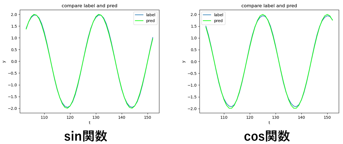
このプログラムを実行すると以下の図をのどちらかをplotしてくれます.(calc_modeの変数でsin関数を予測するのかcos関数を予測するのか選択する必要がある)
この図は,振幅が2,周期が25[s]のsin関数とcos関数の予測結果と正解ラベルを比較している図です.
ほぼほぼ値が一致していることが分かると思います.ただ縦軸が±2付近では少しずれが見られます.
またこの予測結果と正解ラベルのずれの最大値は,sin関数だと0.057418744761889906,cos関数だと0.09099483971649436でした.
3. 単純な数式のクラスの説明
単純な数式をこのクラスで定義します.
私はsin関数とcos関数をここで定義しましたが,ここにどんどん数式を追加で定義していくことでクラスを充実させていくこともできます.
振幅を変えられるようにsin_aやcos_a,周期を変えられるようにsin_tやcos_tという変数を用意しました.
class SimpleFormula():
    def __init__(self, sin_a=2.0, cos_a = 2.0, sin_t=25.0, cos_t = 25.0):
        self.sin_a = sin_a
        self.cos_a = cos_a
        self.sin_t = sin_t
        self.cos_t = cos_t

    def sin(self, input):
        return self.sin_a * np.sin(2.0 * np.pi / self.sin_t * (input))

    def cos(self, input):
        return self.cos_a * np.cos(2.0 * np.pi / self.cos_t * (input))
4. LSTMモデルのクラスの説明
以下のクラスで今回用いたネットワークの構造を定義しています.
このネットワークのモデルはLSTMブロック一つと全結合層1層で構成しました.
sin,cos関数を予測するぐらいの簡単な問題では,これぐらい簡素な構造でもそこそこ良い結果が出ました.
class PredictSimpleFormulaNet(nn.Module):
    def __init__(self, input_size, output_size, hidden_size, batch_first):
        super(PredictSimpleFormulaNet, self).__init__()
        self.rnn = nn.LSTM(input_size = input_size,
                            hidden_size = hidden_size,
                            batch_first = batch_first)
        self.output_layer = nn.Linear(hidden_size, output_size)

        nn.init.xavier_normal_(self.rnn.weight_ih_l0)
        nn.init.orthogonal_(self.rnn.weight_hh_l0)

    def forward(self, inputs):
        h, _= self.rnn(inputs)
        output = self.output_layer(h[:, -1])

        return output
次にクラス内の実装を順番に説明します.
以下のコードは,ネットワークの層や入力サイズなどを定義しています.
nn.LSTMの引数のinput_sizeは,LSTMブロックに入力するデータのサイズのことで,入力したい時系列のサイズではないことに注意してください.
hidden_sizeは,隠れ層のベクトルのサイズ,batch_firstは,LSTMに入力するテンソルの形を決めるためのフラグです.
batch_firstは,デフォルトではFalseで,LSTMに入力するテンソルの形は(時系列のサイズ,バッチサイズ, 入力のサイズ)になります.
Trueにするとテンソルの形は(バッチサイズ,時系列のサイズ,入力のサイズ)となります.
このプログラムのようにバッチを最後に作る場合はTrueにしておくとデータの形を整えやすいです.
class PredictSimpleFormulaNet(nn.Module):
    def __init__(self, input_size, output_size, hidden_size, batch_first):
        super(PredictSimpleFormulaNet, self).__init__()
        self.rnn = nn.LSTM(input_size = input_size,
                            hidden_size = hidden_size,
                            batch_first = batch_first)
        self.output_layer = nn.Linear(hidden_size, output_size)
以下のコードは,重みを初期化している処理をしています.
        nn.init.xavier_normal_(self.rnn.weight_ih_l0)
        nn.init.orthogonal_(self.rnn.weight_hh_l0)
以下のコードは,順伝搬の処理をしています.
self.rnnに渡す引数のinputsのテンソルの形は(バッチサイズ,時系列のサイズ,入力のサイズ)です.(batch_farst=Trueの場合)
sin,cos関数を扱っているため入力サイズと出力はいずれも1です.
バッチサイズが2, 時系列のサイズが3で,sin関数の予測をt0~t3の4つの入力データから学習用に形を整えたい場合,入力を配列風に書くと[[[sin(t0)][sin(t1)][sin(t2)]][[sin(t1)][sin(t2)][sin(t3)]]]となります.
この配列はあくまでも例です.バッチを作る際はランダムに組み合わせを作るので,実際に学習を行うときには,この配列のようにt0~t2の入力データから作った配列の隣にt1~t3の入力データから作った配列が来ることはあまりないと思います.
h, _のhのテンソルの形は,(バッチサイズ,時系列のサイズ,隠れ層のベクトルのサイズ)です.
双方向LSTMを使う場合は(バッチサイズ,時系列のサイズ,隠れ層のベクトルのサイズ×2)になりますが,今回は普通のLSTMを用いるので考えないことにします.
先ほどの[[[sin(t0)][sin(t1)][sin(t2)]][[sin(t1)][sin(t2)][sin(t3)]]]が入力されたとき,hを配列風に書くと[[[h(t0)][h(t1)][h(t2)]][[h(t1)][h(t2)][h(t3)]]]になります.
また_は最後の隠れ層のベクトルとセルのベクトルのタプルです.今回使わないので変数に格納するだけの処理になっています.
そして,最後にLSTMの最後の隠れ層の出力h[:, -1]を全結合層self.output_layerに入力し,予測結果outputを出力します.
この時h[:, -1]のテンソルの形は,(バッチサイズ,隠れ層のベクトルのサイズ)です.
h[:, -1]を配列風に書くと[[[h(t2)]][[h(t3)]]]になります.
    def forward(self, inputs):
        h, _= self.rnn(inputs)
        output = self.output_layer(h[:, -1])

        return output
5. 学習用のクラスの説明
学習用のクラスでは,学習を行うのはもちろんのこと学習のためのデータセット作成や学習したモデルと正解ラベルを比較する関数を定義しています.
学習用のクラスの全体のコード(折りたたんでいるのでこれをクリックして頂けると全体が見られます)
class Train():
    def __init__(self, input_size, output_size, hidden_size, batch_first, lr):
        self.device = torch.device('cuda' if torch.cuda.is_available() else 'cpu')
        print("device:", self.device)
        self.net = PredictSimpleFormulaNet(input_size, output_size, hidden_size, batch_first).to(self.device)
        self.criterion = nn.MSELoss(reduction='mean')
        self.optimizer = optim.Adam(self.net.parameters(), lr=lr, betas=(0.9, 0.999), amsgrad=True)

    def set_formula_const_arg(self, sin_a, cos_a, sin_t, cos_t):
        self.f = SimpleFormula(sin_a, cos_a, sin_t, cos_t)

    def make_dataset(self, dataset_num, sequence_length, t_start, calc_mode="sin"):
        dataset_inputs = []
        dataset_labels = []
        dataset_times = []
        for t in range(dataset_num):
            if calc_mode == "sin":
                dataset_inputs.append([self.f.sin(t_start + t + i) for i in range(sequence_length)])
                dataset_labels.append([self.f.sin(t_start + t + sequence_length)])
            elif calc_mode == "cos":
                dataset_inputs.append([self.f.cos(t_start + t + i) for i in range(sequence_length)])
                dataset_labels.append([self.f.cos(t_start + t + sequence_length)])
            dataset_times.append(t_start + t + sequence_length)
        print("test = {}, {}, {}".format(np.array(dataset_inputs).shape,  np.array(dataset_labels).shape, np.array(dataset_times).shape))
        return np.array(dataset_inputs),  np.array(dataset_labels), np.array(dataset_times)

    def train_step(self, inputs, labels):
        inputs = torch.Tensor(inputs).to(self.device)
        labels = torch.Tensor(labels).to(self.device)
        self.net.train()
        preds = self.net(inputs)
        loss = self.criterion(preds, labels)
        self.optimizer.zero_grad()
        loss.backward()
        # 勾配が大きくなりすぎると計算が不安定になるので、clipで最大でも勾配2.0に留める
        nn.utils.clip_grad_value_(self.net.parameters(), clip_value=2.0)
        self.optimizer.step()

        return loss, preds

    def test_step(self, inputs, labels):
        inputs = torch.Tensor(inputs).to(self.device)
        labels = torch.Tensor(labels).to(self.device)
        self.net.eval()
        preds = self.net(inputs)
        loss = self.criterion(preds, labels)

        return loss, preds

    def train(self, train_inputs, train_labels, test_inputs, test_labels, epochs, batch_size, sequence_length, input_size):
        torch.backends.cudnn.benchmark = True   # ネットワークがある程度固定であれば、高速化させる

        n_batches_train = int(train_inputs.shape[0] / batch_size)
        n_batches_test = int(test_inputs.shape[0] / batch_size)
        for epoch in range(epochs):
            print('-------------')
            print('Epoch {}/{}'.format(epoch+1, epochs))
            print('-------------')
            train_loss = 0.
            test_loss = 0.
            train_inputs_shuffle, train_labels_shuffle = shuffle(train_inputs, train_labels)
            for batch in range(n_batches_train):
                start = batch * batch_size
                end = start + batch_size
                loss, _ = self.train_step(np.array(train_inputs_shuffle[start:end]).reshape(-1, sequence_length, input_size), np.array(train_labels_shuffle[start:end]).reshape(-1, input_size))
                train_loss += loss.item()

            for batch in range(n_batches_test):
                start = batch * batch_size
                end = start + batch_size
                loss, _ = self.test_step(np.array(test_inputs[start:end]).reshape(-1, sequence_length, input_size), np.array(test_labels[start:end]).reshape(-1, input_size))
                test_loss += loss.item()

            train_loss /= float(n_batches_train)
            test_loss /= float(n_batches_test)
            print('loss: {:.3}, test_loss: {:.3}'.format(train_loss, test_loss))

    def pred_result_plt(self, test_inputs, test_labels, test_times, sequence_length, input_size):
        print('-------------')
        print("start predict test!!")
        self.net.eval()
        preds = []
        for i in range(len(test_inputs)):
            input = np.array(test_inputs[i]).reshape(-1, sequence_length, input_size)
            input = torch.Tensor(input).to(self.device)
            pred = self.net(input).data.cpu().numpy()
            preds.append(pred[0].tolist())
        preds = np.array(preds)
        test_labels = np.array(test_labels)
        pred_epss = np.abs(test_labels - preds)
        print("pred_epss_max = {}".format(pred_epss.max()))
        #以下グラフ描画
        plt.plot(test_times, preds)
        plt.plot(test_times, test_labels, c='#00ff00')
        plt.xlabel('t')
        plt.ylabel('y')
        plt.legend(['label', 'pred'])
        plt.title('compare label and pred')
        plt.show()

    def confirm_input_and_label_plot(self, calc_mode, inputs, labels, times):
        #この関数はinputとlabelを可視化するためのコードで基本的に使う必要のない関数です
        print('-------------')
        print("confirm_input_and_label!!")
        re_inputs = inputs[:, -1]
        #以下グラフ描画
        plt.plot(times[:-3], re_inputs[:-3], marker="o")
        plt.plot(times[-3:], re_inputs[-3:], marker="o")
        plt.plot(times[-1]+1.0, labels[-1], marker="o")
        plt.xlabel('t')
        plt.ylabel('y')
        plt.legend([calc_mode, 'input', 'label'])
        plt.title('confirm input and label')
        plt.show()
以下のコードは,ネットワークのモデル,損失関数,最適化手法などを定義しています.
torch.device('cuda' if torch.cuda.is_available() else 'cpu')では,使用可能ならばcudaつまりgpuを使うことを命令しています.
学習はgpuを使ったほうが早いので,使用可能であれば積極的に使うようにしています.
    def __init__(self, input_size, output_size, hidden_size, batch_first, lr):
        self.device = torch.device('cuda' if torch.cuda.is_available() else 'cpu')
        print("device:", self.device)
        self.net = PredictSimpleFormulaNet(input_size, output_size, hidden_size, batch_first).to(self.device)
        self.criterion = nn.MSELoss(reduction='mean')
        self.optimizer = optim.Adam(self.net.parameters(), lr=lr, betas=(0.9, 0.999), amsgrad=True)
以下のコードは,数式のクラスを初期化する関数です.
    def set_formula_const_arg(self, sin_a, cos_a, sin_t, cos_t):
        self.f = SimpleFormula(sin_a, cos_a, sin_t, cos_t)
以下のコードは,学習用のデータセットを作成する関数です.
ここでtrainとtest用のデータセットをまとめて作成し,main文でtrainとtestに分けます.
dataset_numは,作成するデータセットの数,sequence_lengthは,時系列のサイズ,t_startは,データセット作成する初めの時間です.
またcalc_modeで時系列をsin関数で作るのかcos関数で作るのか決めます.
返り値のnp.array(dataset_inputs)の配列の形は,(dataset_num,sequence_length)です.
配列の中身は,[[sin(t0),sin(t1),sin(t2)][sin(t1),sin(t2),sin(t3)]...]です.
このデータは学習用の入力に使います.
返り値のnp.array(dataset_labels)の配列の形は,(dataset_num,ネットワークの出力サイズ)です.
配列の中身は,[sin(t3), sin(t4), ...]です.
このデータは,学習用の正解ラベルに使います.
返り値のnp.array(dataset_times)の配列の形は,(dataset_num,ネットワークの出力サイズ)です.
配列の中身は,[t3, t4, ...]です.
このデータは,trainとtestに分けた後test部分だけをpred_result_pltの関数で使います.
    def make_dataset(self, dataset_num, sequence_length, t_start, calc_mode="sin"):
        dataset_inputs = []
        dataset_labels = []
        dataset_times = []
        for t in range(dataset_num):
            if calc_mode == "sin":
                dataset_inputs.append([self.f.sin(t_start + t + i) for i in range(sequence_length)])
                dataset_labels.append([self.f.sin(t_start + t + sequence_length)])
            elif calc_mode == "cos":
                dataset_inputs.append([self.f.cos(t_start + t + i) for i in range(sequence_length)])
                dataset_labels.append([self.f.cos(t_start + t + sequence_length)])
            dataset_times.append(t_start + t + sequence_length)
        return np.array(dataset_inputs),  np.array(dataset_labels), np.array(dataset_times)
以下のコードは,trainデータの入力と正解ラベルを使ってネットワークのパラメータを更新する処理をしています.
inputsの配列の形は,(バッチサイズ,時系列のサイズ,入力のサイズ)です.
配列の中身は,[[[sin(t0)][sin(t1)][sin(t2)]][[sin(t14)][sin(t15)][sin(t16)]]...]です.
forward関数のところでも言いましたが,バッチはランダムに作るので,t0~t2で作られた入力データの隣の配列は,t1~t3であるとは限りません.上の例のようにt14~t16で作られた入力データの配列かもしれません.
labelsの配列の形は,(バッチサイズ,出力のサイズ)です.
配列の中身は,[[sin(t3)][sin(t17)]...]です.
    def train_step(self, inputs, labels):
        inputs = torch.Tensor(inputs).to(self.device)
        labels = torch.Tensor(labels).to(self.device)
        self.net.train()
        preds = self.net(inputs)
        loss = self.criterion(preds, labels)
        self.optimizer.zero_grad()
        loss.backward()
        # 勾配が大きくなりすぎると計算が不安定になるので、clipで最大でも勾配2.0に留める
        nn.utils.clip_grad_value_(self.net.parameters(), clip_value=2.0)
        self.optimizer.step()

        return loss, preds
以下のコードは,testデータの入力と正解ラベルを使ってlossを計算するだけの処理をしています.
inputsとlabelsの配列の形や中身は,先ほどのtrain_step関数の時と同様です.
    def test_step(self, inputs, labels):
        inputs = torch.Tensor(inputs).to(self.device)
        labels = torch.Tensor(labels).to(self.device)
        self.net.eval()
        preds = self.net(inputs)
        loss = self.criterion(preds, labels)

        return loss, preds
以下のコードは,主にtrainデータのバッチを作る処理とlossを計算する処理を行っています.
train_inputs_shuffle, train_labels_shuffle = shuffle(train_inputs, train_labels)の行の処理では,make_dataset関数で作った順番通りに並んでいる配列の組み合わせをランダムに入れ替えます.
具体的には,train_inputsの配列の中身は,[[sin(t0), sin(t1), sin(t2)][sin(t1), sin(t2), sin(t3)]]...]というように規則正しく順番に並んでいます.
これをtrain_inputs_shuffleの中身では[[sin(t22), sin(t23), sin(t24)][sin(t14), sin(t15), sin(t16)]]...]というようにランダムに入れ替えています.(このインデックス番号は例で,実際どのようにシャッフルされるかは分かりません)
同様にtrain_labelsの配列の中身は,[sin(t3), sin(t4), ...]から[sin(t25), sin(t17), ...]というようにランダムに入れ替えています.
またreshape(-1, sequence_length, input_size)やreshape(-1, input_size)では,ネットワークのモデルの入力の形に合わせる処理を行っています.
具体的には[[sin(t22), sin(t23), sin(t24)][sin(t14), sin(t15), sin(t16)]]...]や[sin(t25), sin(t17), ...]の配列をネットワークのモデルの入力の形に合わせて,[[[sin(t22)][sin(t23)][sin(t24)]][[sin(t14)][sin(t15)][sin(t16)]]...]や[[sin(t25)][sin(t17)]...]に変形させています.
    def train(self, train_inputs, train_labels, test_inputs, test_labels, epochs, batch_size, sequence_length, input_size):
        torch.backends.cudnn.benchmark = True   # ネットワークがある程度固定であれば、高速化させる

        n_batches_train = int(train_inputs.shape[0] / batch_size)
        n_batches_test = int(test_inputs.shape[0] / batch_size)
        for epoch in range(epochs):
            print('-------------')
            print('Epoch {}/{}'.format(epoch+1, epochs))
            print('-------------')
            train_loss = 0.
            test_loss = 0.
            train_inputs_shuffle, train_labels_shuffle = shuffle(train_inputs, train_labels)
            for batch in range(n_batches_train):
                start = batch * batch_size
                end = start + batch_size
                loss, _ = self.train_step(np.array(train_inputs_shuffle[start:end]).reshape(-1, sequence_length, input_size), np.array(train_labels_shuffle[start:end]).reshape(-1, input_size))
                train_loss += loss.item()

            for batch in range(n_batches_test):
                start = batch * batch_size
                end = start + batch_size
                loss, _ = self.test_step(np.array(test_inputs[start:end]).reshape(-1, sequence_length, input_size), np.array(test_labels[start:end]).reshape(-1, input_size))
                test_loss += loss.item()

            train_loss /= float(n_batches_train)
            test_loss /= float(n_batches_test)
            print('loss: {:.3}, test_loss: {:.3}'.format(train_loss, test_loss))
以下のコードは,学習を終えたモデルを使って予測を行い,それを正解ラベルと比較するため可視化する処理を行っています.
    def pred_result_plt(self, test_inputs, test_labels, test_times, sequence_length, input_size):
        print('-------------')
        print("start predict test!!")
        self.net.eval()
        preds = []
        for i in range(len(test_inputs)):
            input = np.array(test_inputs[i]).reshape(-1, sequence_length, input_size)
            input = torch.Tensor(input).to(self.device)
            pred = self.net(input).data.cpu().numpy()
            preds.append(pred[0].tolist())
        preds = np.array(preds)
        test_labels = np.array(test_labels)
        pred_epss = np.abs(test_labels - preds)
        print("pred_epss_max = {}".format(pred_epss.max()))
        #以下グラフ描画
        plt.plot(test_times, preds)
        plt.plot(test_times, test_labels, c='#00ff00')
        plt.xlabel('t')
        plt.ylabel('y')
        plt.legend(['label', 'pred'])
        plt.title('compare label and pred')
        plt.show()
以下のコードは,inputとlabelを可視化するためのコードです.
問題設定のところで使った図を作るための関数で,基本的に使う必要のない関数です
    def confirm_input_and_label_plot(self, calc_mode, inputs, labels, times):
        #この関数はinputとlabelを可視化するためのコードで基本的に使う必要のない関数です
        print('-------------')
        print("confirm_input_and_label!!")
        re_inputs = inputs[:, -1]
        #以下グラフ描画
        plt.plot(times[:-3], re_inputs[:-3], marker="o")
        plt.plot(times[-3:], re_inputs[-3:], marker="o")
        plt.plot(times[-1]+1.0, labels[-1], marker="o")
        plt.xlabel('t')
        plt.ylabel('y')
        plt.legend([calc_mode, 'input', 'label'])
        plt.title('confirm input and label')
        plt.show()
6. main文の説明
main文では,このプログラムで使うほとんどのパラメータを定義しています.
私は使うパラメータをどこか1か所にまとめておくのが好きなのでこのような書き方になっています.
パラメータは頻繁に書き換えるので,この書き方は結構便利だと思います.
後は学習用のクラスの関数を順番に呼び出すだけの処理になっています.
main文の全体のコード(折りたたんでいるのでこれをクリックして頂けると全体が見られます)
if __name__ == '__main__':
    '''
    定数
    '''
    dataset_num = 250
    sequence_length = 3
    t_start = -100.0
    sin_a = 2.0
    cos_a = 2.0
    sin_t = 25.0
    cos_t = 25.0
    calc_mode = "sin"
    # model pram
    input_size = 1
    output_size = 1
    hidden_size = 64
    batch_first = True
    # train pram
    lr = 0.001
    epochs = 15
    batch_size = 4
    test_size = 0.2
    '''
    学習用の関数を呼び出す
    '''
    train = Train(input_size, output_size, hidden_size, batch_first, lr)
    train.set_formula_const_arg(sin_a, cos_a, sin_t, cos_t)
    dataset_inputs, dataset_labels, dataset_times = train.make_dataset(dataset_num, sequence_length, t_start, calc_mode=calc_mode)
    print("dataset_inputs = {}, dataset_labels = {}".format(dataset_inputs.shape, dataset_labels.shape))
    train_inputs, test_inputs, train_labels, test_labels = train_test_split(dataset_inputs, dataset_labels, test_size=test_size, shuffle=False)
    train_times, test_times = train_test_split(dataset_times, test_size=test_size, shuffle=False)
    print("train_inputs = {}, train_labels = {}, test_inputs = {}, test_labels = {}".format(train_inputs.shape, train_labels.shape, test_inputs.shape, test_labels.shape))
    # train.confirm_input_and_label_plot(calc_mode, test_inputs, test_labels, test_times)
    train.train(train_inputs, train_labels, test_inputs, test_labels, epochs, batch_size, sequence_length, input_size)
    train.pred_result_plt(test_inputs, test_labels, test_times, sequence_length, input_size)
6. おわりに
簡単な時系列データを予測するだけでしたが,結構実装するのに苦労しました.
LSTMに限らずCNNなどネットワークに入力するためにデータの形を整えるのは大変ですね...
初めてPyTorchでLSTMの実装をしたので,いろいろ間違った理解や用語の使い方をしているかもしれないので,遠慮なくご指摘頂けると幸いです.
またこの記事で説明したプログラムファイル(predict_simple_formula_train.py)やanacondaの環境ファイル(predict_simple_formula_env.yml)は以下のgithubにもあげているので良かったら見ていってください.
7. 参考にさせていただいたサイト