DNNを用いた画像からジオタグ予測

はじめに

今回は、学習済みモデルを用いて建物画像からジオタグ予測を行いたいと思います。
特に本記事では入力画像から緯度、経度の複数ラベルの出力を使用したいという目的から取り組み始めました。

使用するデータ

今回使用するデータは「European Cities 1M dataset」
http://image.ntua.gr/iva/datasets/ec1m/index.html

このサイトにあるlandmark set imageとgeotagそれぞれ使用します。

構築環境

本記事における実装はGoogle Colaboratoryを用います。
使用した環境の設定を以下に挙げておきます。

• Python3.6.9
• tensorflow 2.3.0
• Keras 2.4.3
• GPU 使用

import keras
from keras.utils import np_utils
from keras.models import Sequential, Model, load_model
from keras.layers.convolutional import Conv2D, MaxPooling2D
from keras.layers.core import Dense, Dropout, Activation, Flatten
import numpy as np
from sklearn.model_selection import train_test_split
import os, zipfile, io, re
from PIL import Image
import glob
from tqdm import tqdm

from sklearn.model_selection import train_test_split
from keras.applications.xception import Xception
from keras.applications.resnet50 import ResNet50
from keras.layers.pooling import GlobalAveragePooling2D
from keras.optimizers import Adam, Nadam

前処理

ここでは前処理として緯度、経度のラベルでの処理を行います。今回はラベルとして緯度、経度を別にして学習するのでリストにして取り出しやすいように処理を行います。

with open("landmark/ec1m_landmarks_geotags.txt") as f:
    label=f.readlines()
    for i in label:
        ans=i.split(' ')
        ans[1]=ans[1].replace('\n','')
        print(ans)

出力

['41.4134', '2.153']
['41.3917', '2.16472']
['41.3954', '2.16177']
['41.3954', '2.16177']
['41.3954', '2.16156']
['41.3899', '2.17428']
['41.3953', '2.16184']
['41.3953', '2.16172']
['41.3981', '2.1645']
.....
.....

データ取得

画像サイズは100とする
データセットを配列に変換
緯度経度を分けないまま画像とラベル付けを行う

X = []
Y = []
image_size=100

with open("landmark/ec1m_landmarks_geotags.txt") as f:
    label=f.readlines()

    dir = "landmark/ec1m_landmark_images"
    files = glob.glob(dir + "/*.jpg")
    for index,file in tqdm(enumerate(files)):
        image = Image.open(file)
        image = image.convert("RGB")
        image = image.resize((image_size, image_size))
        data = np.asarray(image)
        X.append(data)
        Y.append(label[index])
 
X = np.array(X)
Y = np.array(Y)

出力

927it [00:08, 115.29it/s]

それぞれの形状はこのようになっている

X.shape,Y.shape
((927, 100, 100, 3), (927,))

次にtrain,test,validに分割を行う
ここで緯度、経度の分割も行う

y0=[]  #緯度ラベル
y1=[]  #経度ラベル

for i in Y:
    ans=i.split(' ')
    ans[1]=ans[1].replace('\n','')
    y0.append(float(ans[0]))
    y1.append(float(ans[1]))

y0=np.array(y0)
y1=np.array(y1)

# xの(train,test)分割
X_train, X_test = train_test_split(X, random_state = 0, test_size = 0.2)
print(X_train.shape,  X_test.shape) 

# (741, 100, 100, 3) (186, 100, 100, 3)

# y0,y1の(train,test)分割
y_train0,y_test0,y_train1, y_test1 = train_test_split(y0,y1,
                                                      random_state = 0,
                                                      test_size = 0.2)
print(y_train0.shape,  y_test0.shape) 
print(y_train1.shape,  y_test1.shape)

# (741,) (186,)
# (741,) (186,)

# データ型の変換＆正規化
X_train = X_train.astype('float32') / 255
X_test = X_test.astype('float32') / 255

# xの(train,valid)分割
X_train, X_valid= train_test_split(X_train, random_state = 0, test_size = 0.2)
print(X_train.shape,  X_valid.shape) 

# (592, 100, 100, 3) (149, 100, 100, 3)

# y0,y1の(train,valid)分割
y_train0, y_valid0,y_train1, y_valid1= train_test_split(y_train0,y_train1,
                                                        random_state = 0,
                                                        test_size = 0.2)

print(y_train0.shape,  y_valid0.shape) 
print(y_train1.shape,  y_valid1.shape) 

# (592,) (149,)
# (592,) (149,)

モデル構築

今回は以下の記事を参考にXceptionの学習済みモデルを用いる
https://qiita.com/ha9kberry/items/314afb56ee7484c53e6f#データ取得

ほかのモデルでも試してみたかったのでResnetも使用してみる

# xception model
base_model = Xception(
    include_top = False,
    weights = "imagenet",
    input_shape = None
)

# resnet model
base_model = ResNet50(
    include_top = False,
    weights = "imagenet",
    input_shape = None
)

回帰問題より最後に予測値を１つ入力する
緯度、経度のラベル出力を用意する

x = base_model.output
x = GlobalAveragePooling2D()(x)
x = Dense(1024, activation='relu')(x)
predictions1 = Dense(1,name='latitude')(x)
predictions2 = Dense(1,name='longitude')(x)

outputにpredictions1,predictions2を入れる。
他は参考記事の通り
今回はオプティマイザにAdamとNadamを用いて学習を行う。

model = Model(inputs = base_model.input, outputs = [predictions1,predictions2])

# 108層までfreeze
for layer in model.layers[:108]:
    layer.trainable = False

    # Batch Normalizationのfreeze解除
    if layer.name.startswith('batch_normalization'):
        layer.trainable = True
    if layer.name.endswith('bn'):
        layer.trainable = True

# 109層以降、学習させる
for layer in model.layers[108:]:
    layer.trainable = True

# layer.trainableの設定後にcompile
model.compile(
    optimizer = Adam(),
    #optimizer=Nadam(),
    loss = {'latitude':root_mean_squared_error,
            'longitude':root_mean_squared_error
        }
)

学習

history = model.fit( X_train,   #decode_train
                    {'latitude': y_train0,
                     'longitude':y_train1},
                    batch_size=64,
                    epochs=50,
                    validation_data=(X_valid,    decode_valid
                                     {'latitude' :y_valid0,
                                      'longitude':y_valid1}),
                    )

出力

Epoch 1/50
10/10 [==============================] - 4s 409ms/step - loss: 0.6146 - latitude_loss: 0.4365 - longitude_loss: 0.1782 - val_loss: 1.6756 - val_latitude_loss: 1.3430 - val_longitude_loss: 0.3326
Epoch 2/50
10/10 [==============================] - 4s 404ms/step - loss: 0.5976 - latitude_loss: 0.4415 - longitude_loss: 0.1562 - val_loss: 0.7195 - val_latitude_loss: 0.5987 - val_longitude_loss: 0.1208

...
...

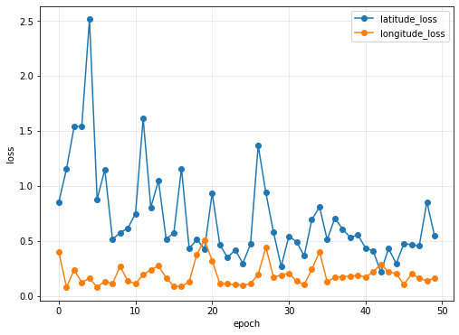
結果をプロット

import matplotlib.pyplot as plt


plt.figure(figsize=(18,6))

# loss
plt.subplot(1, 2, 1)
plt.plot(history.history["latitude_loss"], label="latitude_loss", marker="o")
plt.plot(history.history["longitude_loss"], label="longitude_loss", marker="o")
# plt.yticks(np.arange())
# plt.xticks(np.arange())
plt.ylabel("loss")
plt.xlabel("epoch")
plt.title("")
plt.legend(loc="best")
plt.grid(color='gray', alpha=0.2)

plt.show()

結果

評価

# batch size 64  Adam
scores = model.evaluate(X_test,{'latitude' :y_test0,
                                'longitude':y_test1}, 
                             verbose=1)

print("total loss:\t{0}".format(scores[0]))
print("latitude loss:\t{0}".format(scores[1]))
print("longtitude loss:{0}".format(scores[2]))

出力

total loss:	0.7182420492172241
latitude loss:	0.6623533964157104
longtitude loss:0.05588864907622337

予測

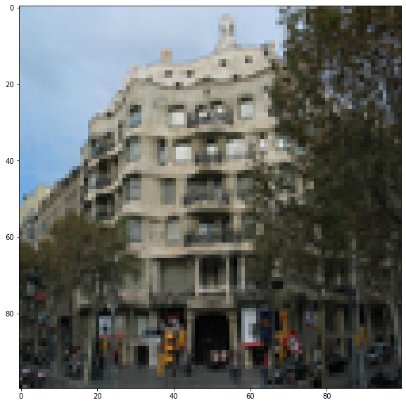
# show image, prediction and actual label
for i in range(10,12):
    plt.figure(figsize=(10,10))
    print('latitude:{} \tlongititude{}'.format(
        prediction[0][i],
        prediction[1][i],
        ))

    plt.imshow(X_test[i].reshape(100, 100, 3))
    plt.show()

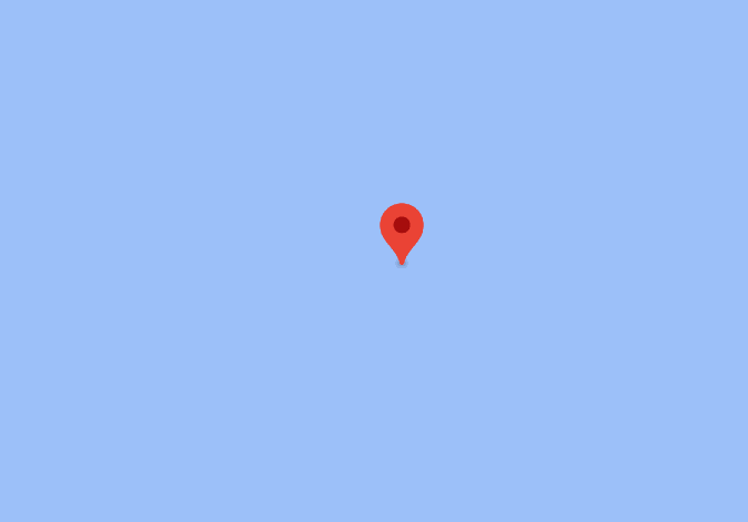
latitude:[39.69221] longititude[2.2188098]

latitude:[39.728386] longititude[2.224149]

それっぽい数値が出ているが、地図上(GoogleMap)で表すと以下のように海の真ん中になっており、使用するには不十分だろう

他のパラメータでの比較

使用パラメータ	Total loss	latitude_loss	longtitude_loss
Xception , Adam	0.7182	0.6623	0.0558
Xception , Nadam	0.3768	0.1822	0.1946
Resnet , Adam	0.7848	0.7360	0.0488
Resnet , Nadam	49.6434	47.2652	2.3782
Resnet,Adam,AutoEncoder	1.8299	1.6918	0.13807

さいごに

今回の試行ではXception,Nadamの組み合わせが一番精度が高いことが分かった
今後は他のモデルを使用するか、一からモデルを作成しようと思う

参考、引用

データセット

Publications
Conferences
Y. Avrithis, Y. Kalantidis, G. Tolias, E. Spyrou. Retrieving Landmark and Non-Landmark Images from Community Photo Collections. In Proceedings of ACM Multimedia (MM 2010), Firenze, Italy, October 2010.

Journals
Y. Kalantidis, G. Tolias, Y. Avrithis, M. Phinikettos, E. Spyrou, P. Mylonas, S. Kollias. VIRaL: Visual Image Retrieval and Localization. In Multimedia Tools and Applications (to appear), 2011.

記事

• https://qiita.com/ha9kberry/items/314afb56ee7484c53e6f#概要
• https://qiita.com/cvusk/items/1439c1c6dde160c48d13