AutoML vs 俺 －真剣二番勝負－

※こちらは塩尻MLもくもく会 #13の発表資料です。

タイトルは大げさに書いております。

先日、機械学習プロセスの自動化を行う「AutoML」の紹介記事が公開されました。
https://qiita.com/Hironsan/items/30fe09c85da8a28ebd63

そこで、本稿ではAutoMLと私を対決をさせてみました。

AutoMLとは

• イメージでいうと、ターミネーターのイメージネットみたいな凄いヤツです。
• 機械学習で面倒くさい作業（モデル選択、ハイパーパラメータのチューニング、特徴エンジニアリングなど）を自動でやってくれます。
• 詳細は冒頭に紹介した記事をご覧ください。

俺とは

• 私のことです。
• Kaggleにも参加したことがない未熟者です。
• 一人ぼっちだと心細いので、今回はベイズ最適化という武器を使います。

ルール

AutoML陣営

• モデル選択とハイパーパラメータのチューニングは各種AutoMLを使います。
• 今回は、特徴エンジニアリングは行いません。

俺陣営

• モデル選択は、私の独断と偏見で一つに絞ります。
• ただし、ハイパーパラメータ探索はベイズ最適化を使うこともあります。
• こちらも特徴エンジニアリングは行いません。
• Data Augmentation（データの水増し）も行いません。
• 転移学習やFine-tuningも行いません。
• 学習を始めたら、やり直しが効かない一発勝負です。

分類勝負

まずは、CIFAR10の画像で分類勝負を行います。

画像の大きさ	クラス数	訓練データ数	テストデータ数
32×32	10	50,000	10,000

AutoMLの作戦

• 画像といえば、ニューラルネットワークで決まり！
• ということで、Auto-Kerasを使います。

import autokeras as ak
from keras.datasets import cifar10

# データの読み込み
(X_train, y_train), (X_test, y_test) = cifar10.load_data()
X_train, X_test = X_train / 255.0, X_test / 255.0

#学習と結果の表示
clf = ak.ImageClassifier(verbose=True)
clf.fit(X_train, y_train, time_limit=10 * 60 * 60)
clf.final_fit(X_train, y_train, X_test, y_test, retrain=True)
print(clf.evaluate(X_test, y_test))

コードはこれだけ！驚きです。

俺の作戦

• 当然、畳み込みニューラルネットワークを使います。
• 畳込み層が32層のRes-net32ライクなネットワークを構築してみました。
• コードは「付録」に記載しました。

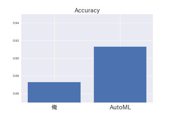
結果の比較

まずは、俺の結果から

Epoch 159/200
50000/50000 [============] - 161s 3ms/step - loss: 0.0072 - acc: 0.9979 - val_loss: 0.7334 - val_acc: 0.8732

分類精度は0.873でした。
まずまずの結果といえます。

続いて、AutoMLの結果は

+--------------------------------------------------------------------------+
|    Father Model ID     |                 Added Operation                 |
+--------------------------------------------------------------------------+
|           5            |    to_deeper_model 25 Conv2d(128, 128, 5, 1)    |
+--------------------------------------------------------------------------+

Saving model.
+--------------------------------------------------------------------------+
|        Model ID        |          Loss          |      Metric Value      |
+--------------------------------------------------------------------------+
|           6            |   1.0844052225351333   |         0.9132         |
+--------------------------------------------------------------------------+

分類精度は0.913でした。

Data Augmentationを使わずに精度0.9を超えるとは驚愕です。
AutoMLの強さを見せつけられました。

回帰勝負

気を取り直して、ボストンハウスのデータセットで回帰勝負を行います。

説明変数の数	出力	訓練データ数	テストデータ数
13	住宅の価格	404	102

事前に、学習データとテストデータを分けておきます。

from sklearn.datasets import load_boston
from sklearn.model_selection import train_test_split

digits = load_boston()
x_train, x_test, y_train, y_test = train_test_split(digits.data, digits.target,
                                                    train_size=0.8, test_size=0.2)

精度の比較はMSEを使っても良いですが、今回は相関係数を使いました。

AutoMLの作戦

• テーブルデータの分析は、決定木やロッソ回帰など多様なモデルが活躍しそうです。
• ということで、TPOTを使います。TPOTの回帰はこちらの記事に使い方が書かれています。

from tpot import TPOTRegressor
import numpy as np

#学習
tpot = TPOTRegressor(max_time_mins=6*60, verbosity=2)
tpot.fit(x_train, y_train)

#結果の表示
y_pred = tpot.predict(x_test)
R = np.corrcoef(y_test, y_pred)
print("R is ",R[0,1])

コードは数行です。またまた驚きました。

俺の作戦

• ちょっと古いですが、XGBoostを使いました。
• ハイパーパラメーターの探索はベイズ最適化を使いました。
• コードは「付録」に記載しました。

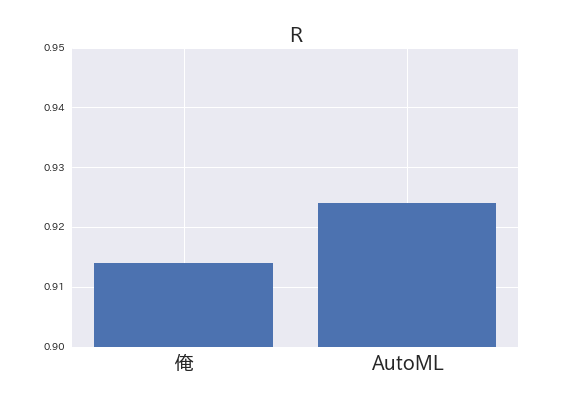
結果の比較

まずは、俺の結果から

R is  0.9138793118926807

相関係数は0.914でした。

相関係数の最大値は1です。そして、これは大きければ大きいほど良いモデルといえます。
0.9を超えてきたのは、まずまずといったところです。

続いてAutoMLの結果は

R is  0.9236799830997592

相関係数は0.924でした。
回帰勝負でもAutoMLが勝ちました。

まとめ

• 予想はしていましたが、AutoMLの圧勝でした。AutoML凄い！
• AutoMLを使えば「コードは数行」、「精度が出る」と良いことづくめです。
• 皆さんも是非使ってみてください。

付録

俺のコード（分類勝負）

演算はColaboratoryのTPUを使っています。

import tensorflow as tf
import tensorflow.keras.backend as K

from tensorflow.keras.layers import Input, Conv2D, GlobalAveragePooling2D, BatchNormalization
from tensorflow.keras.layers import Add, Activation, Dense
from tensorflow.keras.models import Model
from tensorflow.keras.datasets import cifar10
from tensorflow.keras.utils import to_categorical
from tensorflow.contrib.tpu.python.tpu import keras_support

import numpy as np
import matplotlib.pyplot as plt
import os


# データの読み込み
(X_train, y_train), (X_test, y_test) = cifar10.load_data()
X_train, X_test = X_train / 255.0, X_test / 255.0
y_train, y_test = to_categorical(y_train), to_categorical(y_test)

#res block
def resblock(x, filters, kernel_size):
    x_ = Conv2D(filters, kernel_size, padding='same')(x)
    x_ = BatchNormalization()(x_)
    x_ = Activation("relu")(x_)
    x_ = Conv2D(filters, kernel_size, padding='same')(x_)
    x = Add()([x_, x])
    x = BatchNormalization()(x)
    x = Activation("relu")(x)
    return x

#cnnの構築
input_ = Input(shape=(32, 32, 3))#横の数、縦の数、RGB

c = Conv2D(64, (1, 1), padding="same")(input_)
c = BatchNormalization()(c)
c = Activation("relu")(c)
c = resblock(c,filters=64, kernel_size=(3, 3))
c = resblock(c,filters=64, kernel_size=(3, 3))
c = resblock(c,filters=64, kernel_size=(3, 3))

c = Conv2D(128, (3, 3), strides=2)(c)
c = BatchNormalization()(c)
c = Activation("relu")(c)
c = resblock(c,filters=128, kernel_size=(3, 3))
c = resblock(c,filters=128, kernel_size=(3, 3))
c = resblock(c,filters=128, kernel_size=(3, 3))
c = resblock(c,filters=128, kernel_size=(3, 3))

c = Conv2D(256, (3, 3), strides=2)(c)
c = BatchNormalization()(c)
c = Activation("relu")(c)
c = resblock(c,filters=256, kernel_size=(3, 3))
c = resblock(c,filters=256, kernel_size=(3, 3))
c = resblock(c,filters=256, kernel_size=(3, 3))
c = resblock(c,filters=256, kernel_size=(3, 3))
c = resblock(c,filters=256, kernel_size=(3, 3))

c = Conv2D(512, (3, 3), strides=2)(c)
c = BatchNormalization()(c)
c = Activation("relu")(c)
c = resblock(c,filters=512, kernel_size=(3, 3))
c = resblock(c,filters=512, kernel_size=(3, 3))

c = GlobalAveragePooling2D()(c)
c = Dense(10, activation='softmax')(c)

model = Model(input_, c)

model.compile(tf.train.AdamOptimizer(), loss="categorical_crossentropy", metrics=["acc"])

# TPU
tpu_grpc_url = "grpc://"+os.environ["COLAB_TPU_ADDR"]
tpu_cluster_resolver = tf.contrib.cluster_resolver.TPUClusterResolver(tpu_grpc_url)
strategy = keras_support.TPUDistributionStrategy(tpu_cluster_resolver)
model = tf.contrib.tpu.keras_to_tpu_model(model, strategy=strategy)

#cnnの学習
model.fit(X_train, y_train, batch_size=128, epochs=10, verbose=1)

俺のコード（回帰勝負）

演算は30分くらい（CPU）で終わります。

import xgboost as xgb
import numpy as np
import GPy
import GPyOpt
from sklearn.metrics import accuracy_score
from sklearn.model_selection import KFold
from sklearn.model_selection import cross_val_score

def f(x):
    model = xgb.XGBRegressor( eta = float(x[:,0]),
                              max_depth = int(x[:,1]),
                              min_child_weight = float(x[:,2]),
                              subsample = float(x[:,3]),
                              colsample_bytree = float(x[:,4]),
                              gamma = float(x[:,5]),
                              n_estimators = int(x[:,6]),
                              learning_rate = float(x[:,7]),
                              reg_lambda = float(x[:,8]),
                              reg_alpha = float(x[:,9]),
                              num_boost_round = int(x[:,10]))

    # CV
    kfold = KFold(n_splits=10, random_state=7)
    result = cross_val_score(model, x_train, y_train, cv=kfold)
    score = np.mean(result)
    print(score)

    return -score

bounds = [{'name': 'eta', 'type': 'continuous', 'domain': (0,5)},
          {'name': 'max_depth', 'type': 'continuous', 'domain': (100,250)},
          {'name': 'min_child_weight', 'type': 'continuous', 'domain': (1,5)},
          {'name': 'subsample', 'type': 'continuous', 'domain': (0,1)},
          {'name': 'colsample_bytree', 'type': 'continuous', 'domain': (0.1,1)},
          {'name': 'gamma', 'type': 'continuous', 'domain': (0,2)},
          {'name': 'n_estimators', 'type': 'continuous', 'domain': (10,50)},
          {'name': 'learning_rate', 'type': 'continuous', 'domain': (0,1)},
          {'name': 'reg_lambda', 'type': 'continuous', 'domain': (0,1.1)},
          {'name': 'reg_alpha', 'type': 'continuous', 'domain': (0,1.1)},
          {'name': 'num_boost_round', 'type': 'continuous', 'domain': (200,400)}]

print("Bayesian Optimization")
myBopt = GPyOpt.methods.BayesianOptimization(f=f, domain=bounds)
myBopt.run_optimization(max_iter=200)

#最適なパラメータの表示
print("best parameters =")
print(myBopt.x_opt)

#最適なパラメータで再度学習
x = myBopt.x_opt
Xgb = xgb.XGBRegressor(eta=x[0], max_depth=int(x[1]),min_child_weight=x[2],
                        subsample=x[3], colsample_bytree=x[4], gamma=x[5], n_estimators=int(x[6]),
                        learning_rate=x[7], reg_lambda=x[8], reg_alpha=x[9],num_boost_round=int(x[10]))
Xgb.fit(x_train,y_train)

#結果表示
y_pred = Xgb.predict(x_test)
R = np.corrcoef(y_test, y_pred)
print("R is ",R[0,1])