ディープラーニングで7月の気温を分析（1） －LSTM－

今年の7月は、例年より暑い日が続いているような気がします。
そこでディープラーニングを使って、最高気温の推移を分析しました。

まずは可視化

気象庁のサイトからデータを入手します。
http://www.data.jma.go.jp/gmd/risk/obsdl/index.php

今回は、松本市（7月1日～20日）の30年分の最高気温を使います。
そして、学習データとテストデータを以下のように分けます。
・学習データ：1989年～2008年
・テストデータ：2009年～2018年

学習データとテストデータを可視化してみます。

import matplotlib.pyplot as plt
import matplotlib.cm as cm
import numpy as np

#30年分の　温度データロード,整列
X = np.loadtxt("temperature.csv",delimiter=",")
data = X[:20]
for i in range(1,30):
    x = X[i*20:i*20+20]
    data = np.vstack((data,x))

#テストデータと学習データの分割
x_train = data[:20]
x_test = data[20:]

#可視化
plt.figure()
for i in range(len(x_train)):
    year = 1989+i
    plt.plot(range(1,21),x_train[i], color=cm.jet(float(i) /len(x_train)),label=year)
#plt.legend(loc="lower right")
plt.title("Training data")
plt.ylim(15,40)
plt.xlabel("date")
plt.ylabel("temperature")
plt.show()

plt.figure()
for i in range(len(x_test)):
    year = 2009+i
    plt.plot(range(1,21),x_test[i], color=cm.jet(float(i) / len(x_test)),label=year)
plt.legend(loc="lower right")
plt.title("Test data")
plt.ylim(15,40)
plt.xlabel("date")
plt.ylabel("temperature")
plt.show()

学習データはこちら↓

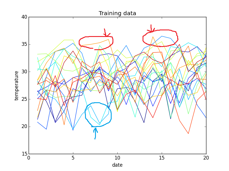
上のグラフの縦軸は気温（℃）、横軸は日付（左端は7/1、右端は7/20）です。

ごちゃごちゃして分かりにくいですが、低温域と高温域の傾向を見てみます。
・低温域では、23℃以下の日は連続しても3日ほどです（青い丸）。
・高温域では、33℃以上の日は連続しても5日ほどです（赤い丸）。

テストデータはこちら↓

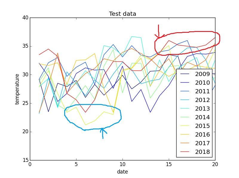
テストデータもザッっと見てみます。
・2018年は、33℃以上の日が7日ほど続いています（赤い丸）。
　明らかに例年の傾向から外れている気がします。
・2015年では、低温が連続しているのも気になるところです（青い丸）。

本稿では、こういった例年の傾向から外れているものを検出させたいと思います。
具体的には、気温の推移が確率的にどのくらいあり得るのかをLSTMを使って数値化します。

問題設定

時系列データを取り扱うに当たり、以下の図のような問題を考えます。

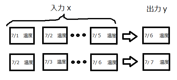
過去5日分の気温推移から次の日の気温を予測するものです。
そして、出力yを以下のクラスに割り当てます。

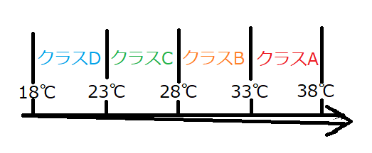
全体として、以下のシステムを構築します。

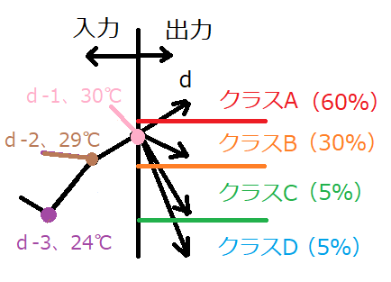
d-5日からd-1日の気温を判別モデルに入力し、d日の気温クラスを予測するものです。

上の例の場合、クラスAとBは確率的にあり得ますが、クラスCとDになった場合、
例年より傾向がズレていると言えそうです。言うなれば、異常検知です。
ここのアイデアは異常検知ナイト（再生場所40：00くらい）を参考にさせていただきました。

本稿では、判別モデルとしてLSTMを用いました。
LSTMについて知りたい方は以下の記事を参考にしてください。
https://qiita.com/KojiOhki/items/89cd7b69a8a6239d67ca

モデル構築

まずは、時系列データを作ります。
過学習を監視するためにValidationデータも作っています。

#LSTMデータの作成
from sklearn.cross_validation import train_test_split
#新バージョンはfrom sklearn.cross_model_selection
from keras.utils import to_categorical

#LSTMデータの作成
def make_data(x_train_rnn,Lookback=5):
    data, target = [], []

    for i in range(x_train_rnn.shape[0]):
        for j in range(x_train_rnn.shape[1]-Lookback):
            data.append(x_train_rnn[i,j:j+Lookback])

            if x_train_rnn[i,j+Lookback] >33:
                label = 0
            elif x_train_rnn[i,j+Lookback] >28:
                label = 1
            elif x_train_rnn[i,j+Lookback] >23:
                label = 2
            else:
                label = 3
            target.append(label)

    re_data = np.array(data).reshape(len(data), Lookback, 1)
    #re_target = np.array(target).reshape(len(data), 1)
    re_target = target

    return re_data, re_target

x_train,y_train = make_data(x_train0)
y_train = to_categorical(y_train)

#trainとvalidationを分割
X_train, X_val, Y_train, Y_val = train_test_split(x_train, y_train, test_size=0.2)

X_test,Y_test = make_data(x_test0)
Y_test = to_categorical(Y_test)

#入力が0~1になるように修正
x_max = np.max(X_train)
x_min = np.min(X_train)

X_train = (X_train-x_min)/(x_max-x_min)
X_val = (X_val-x_min)/(x_max-x_min)
X_test = (X_test-x_min)/(x_max-x_min)

kerasを使ってLSTMを構築します。

#LSTMの学習
from keras.models import Sequential
from keras.layers import Dense, Activation, Dropout
from keras.layers.recurrent import LSTM

lookback = 5

#LSTMの学習
model = Sequential()
model.add(LSTM(20, batch_input_shape=(None,lookback,1)))
model.add(Dropout(0.1))
model.add(Dense(4))
model.add(Activation('softmax'))

model.compile(loss='categorical_crossentropy',
              optimizer='adam',
              metrics=['accuracy'])

hist = model.fit(X_train, Y_train, batch_size = 10, epochs=200, verbose=1, shuffle=True,
                 validation_data = (X_val,Y_val))

#結果描画
plt.figure()               
plt.plot(hist.history['val_loss'],label="val_loss")
plt.plot(hist.history['loss'],label="train_loss")
plt.legend()
plt.show()

plt.figure()               
plt.plot(hist.history['val_acc'],label="val_acc")
plt.plot(hist.history['acc'],label="train_acc")
plt.legend(loc="lower right")
plt.show()

学習結果は以下のとおりです。
損失関数の推移↓

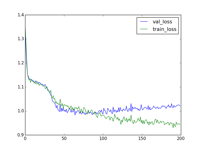
精度の推移↓

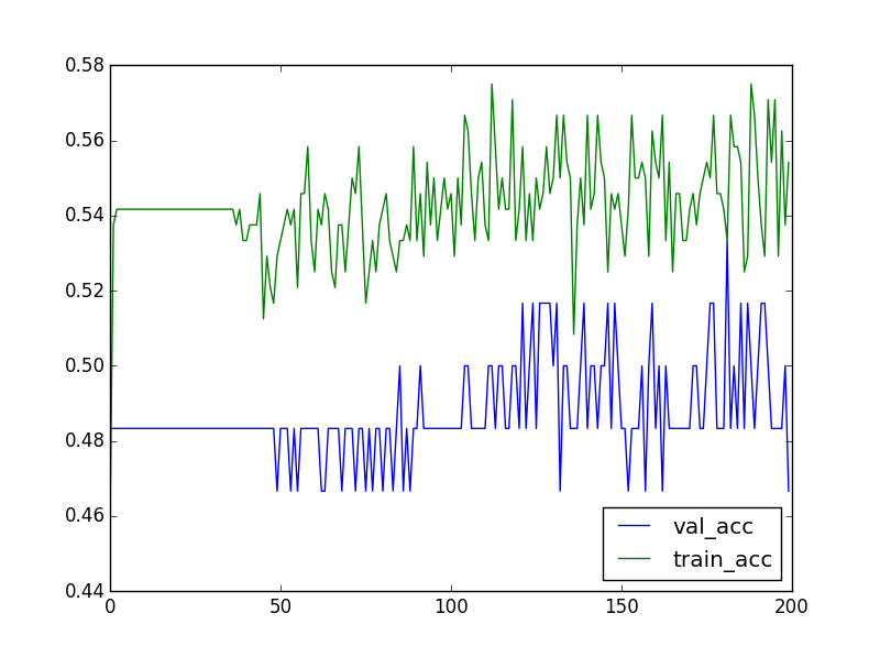
trainデータの精度は55％ほどでした。
明らかにうまくいってない気がしますが、そこは次回改良したいと思います。

評価

テストデータで確率を出してみます。

#正解ラベル
test_label = []
for i in range(len(Y_test)):
    test_label.append(np.argmax(Y_test[i]))

#確率算出
result = model.predict(X_test)
result_prob = []
for i in range(len(result)):
    temp = result[i,test_label[i]]
    result_prob.append(temp)

#確率抽出
graph = result_prob[:15]
for i in range(1,10):
    temp = result_prob[i*15:i*15+15]
    graph = np.vstack((graph,temp))

#確率描画
plt.figure()
for i in range(len(graph)):
    year = 2009+i
    plt.plot(range(6,21),graph[i], color=cm.jet(float(i) / len(graph)),label=year)
plt.legend(loc="lower right")
plt.title("Test data")
plt.xlabel("date")
plt.ylabel("Probability")
plt.show()

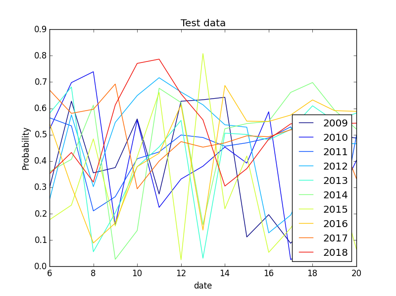
上のグラフは、その日の最高気温が確率的にどのくらいあり得るのかを示したものです。
全体的に40％以上の確率になっています。しかし、これだけではよく分かりません。

気温データの推移と共に可視化します。

#確率0.2以下を描画
plot_anomaly_x = []
plot_anomaly_y = []

for i in range(graph.shape[0]):
    for j in range(graph.shape[1]):
        if graph[i,j] < 0.2:
            plot_anomaly_x.append(j+lookback+1)
            plot_anomaly_y.append(x_test0[i,j+5])

plt.figure()
for i in range(len(x_test0)):
    year = 2009+i
    plt.plot(range(1,21),x_test0[i], color=cm.jet(float(i) / len(x_test0)),label=year)
#plt.legend(loc="lower right")
plt.scatter(np.array(plot_anomaly_x),np.array(plot_anomaly_y),c="r")
plt.title("Test data")
plt.ylim(20,40)
plt.xlim(5,20)
plt.xlabel("date")
plt.ylabel("temperature")
plt.show()

下のグラフの縦軸は気温（℃）、横軸は日付（左端は7/5、右端は7/20）です。
・折れ線はその日の最高気温を示しています。
・赤い丸はLSTMの確率が20％を下回るものをプロットしています。
　つまり、異常と認識している点です。

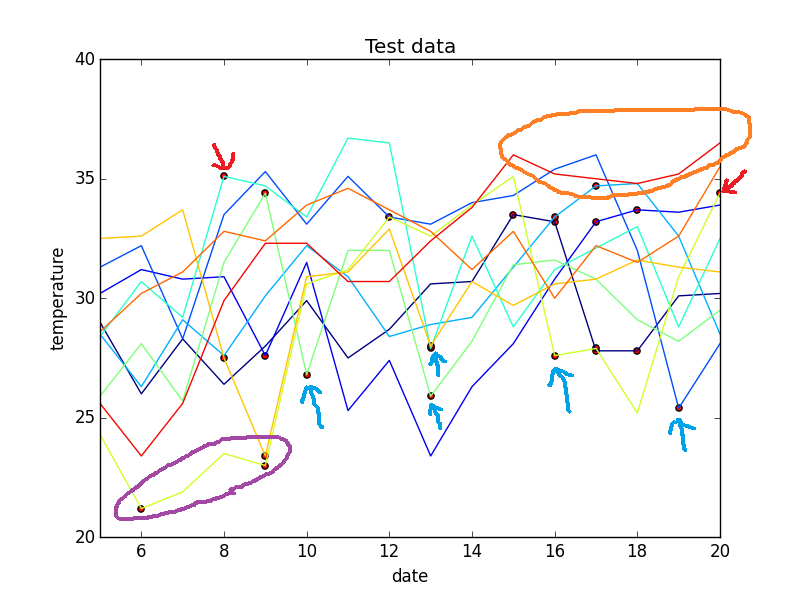
以下、考察を示します。
（良かったところ）
・最高気温が急降下しているものは、確率が低いようです。（青い矢印）
　感覚的に「今日の最高気温は昨日より10℃下がる」と言われたら驚くと思います。
　従って、ここはうまく検出できていると思います。

・最高気温が急上昇しているものも、確率が低いようです。（赤い矢印）
　これはさきほどの裏返しですね。ここもうまく検出できていると思います。

・低温が続くのも確率が低いようです。（紫の丸）
　冒頭で述べたように2015年で低温が続くのは、明らかに例年から
　ズレているように思えましたので、これもうまく検出できていると思います。

（悪かったところ）
・肝心の2018年の高温は検出できませんでした。（オレンジの丸）

次回はCNNを使って改善したいと思います。