初めに
Deep Neural Networkを設計する際、
・隠れ層は何層がいいのか?
・ニューロン数はいくつがいいのか?
・活性化関数は何が良いのか?
・batch,epochsはどのくらいがよい?
etc...
ハイパーパラメータのチューニングが必要になってくる。
そんな時にGrid Searchを活用すれば、計算コストは増加するが
人間の作業は効率化できる。
本記事では、TensorflowとGridSearchを活用した内容について記述したいと思います。
データセットについて
本記事では回帰問題のDNNのハイパーパラメータのチューニングに関する内容とするため、
データセットは前回記事のデータセットを活用する。
サンプルコード
# ライブラリのインポート
import pandas as pd
import numpy as np
from sklearn.datasets import fetch_california_housing
cali_housing = fetch_california_housing(as_frame=True)
x=cali_housing.data
y=cali_housing.target
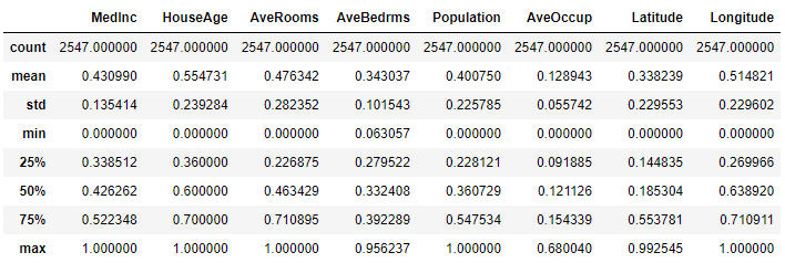
cali_housing.frame.describe()
df=cali_housing.frame
ar_std=df['AveRooms'].std()
ab_std=df['AveBedrms'].std()
pop_std=df['Population'].std()
ao_std=df['AveOccup'].std()
mhv_std=df['MedHouseVal'].std()
ar_mean=df['AveRooms'].mean()
ab_mean=df['AveBedrms'].mean()
pop_mean=df['Population'].mean()
ao_mean=df['AveOccup'].mean()
mhv_mean=df['MedHouseVal'].mean()
limit_low=ar_mean - 1*ab_std
limit_high=ar_mean + 1*ab_std
limit_low1=ab_mean - 1*ab_std
limit_high1=ab_mean + 1*ab_std
limit_low2=pop_mean - 1*pop_std
limit_high2=pop_mean + 1*pop_std
limit_low3=ao_mean - 1*ao_std
limit_high3=ao_mean + 1*ao_std
limit_low4=mhv_mean -1*mhv_std
limit_high4=mhv_mean +1*mhv_std
newdf=df.query('@limit_low < AveRooms < @limit_high')
newdf1=newdf.query('@limit_low1 < AveBedrms < @limit_high1')
newdf2=newdf1.query('@limit_low2 < Population < @limit_high2')
newdf3=newdf2.query('@limit_low3 < AveOccup < @limit_high3')
newdf4=newdf3.query('@limit_low4 < MedHouseVal < @limit_high4')
newdf4.describe()
#正規化(Max-Min法)
def minmax_norm(df):
return (df - df.min()) / ( df.max() - df.min())
df_minmax_norm = minmax_norm(newdf4)
df_minmax_norm.describe()
# 必要なライブラリーのインポート
import seaborn as sns
# 多変量連関図
sns.pairplot(df_minmax_norm, size=1.0)
#データ分け
x=df_minmax_norm.iloc[:,0:8]
y=df_minmax_norm.iloc[:,8:9]
from sklearn.model_selection import train_test_split
#全体データから未知データを生成
x_know,x_unknown,y_know,y_unknown=train_test_split(x,y,test_size=0.2)
#既知データから訓練データとテストデータに分割
x_train,x_test,y_train,y_test=train_test_split(x_know,y_know,test_size=0.2)
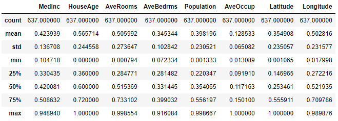
Testデータは下図の通りです。
データ数は637
ハイパーパラメータのチューニングについて
それでは本題です。
ライブラリをインポートします
# Importing the necessary packages
from sklearn.model_selection import GridSearchCV, KFold
from keras.models import Sequential
from keras.layers import Dense
#分類問題用のライブラリ
#from keras.wrappers.scikit_learn import KerasClassifier
#回帰問題用のライブラリ
from keras.wrappers.scikit_learn import KerasRegressor
from keras.optimizers import Adam
from keras.layers import Dropout
グリッドサーチができるようにDNNの定義をします
| 因子 | 1水準目 | 2水準目 |
|---|---|---|
| 学習率 | 0.1 | 0.5 |
| epochs | 100 | 300 |
| batchサイズ | 50 | 100 |
のチューニングを例に書きます。
# DNNモデル定義
def create_model(learning_rate):
    model = Sequential()
    model.add(Dense(64,input_dim = 8,kernel_initializer = 'normal',activation = 'relu'))
    model.add(Dense(32,activation = 'relu'))
    model.add(Dense(16,activation = 'relu'))
    model.add(Dense(8,activation = 'relu'))
    model.add(Dense(1,activation = 'linear'))

    adam = Adam(lr = learning_rate)
    #model.compile(loss = 'binary_crossentropy',optimizer = adam,metrics = ['acc'])
    model.compile(loss = 'rmse',optimizer = adam,metrics = ['mae'])
    return model

# Create the model
#model = KerasClassifier(build_fn = create_model,verbose = 0,batch_size = 40,epochs = 10)

# Define the grid search parameters
epochs_grid=[100,300]
batch_size_grid=[50,100]
learning_rate = [0.1,0.5]

### the grid search parametersを辞書型で定義する
param_grids = dict(learning_rate = learning_rate,batch_size=batch_size_grid,epochs=epochs_grid)

#参考:分類問題の設定
#model = KerasClassifier(build_fn = create_model,verbose = 0,batch_size = batch_size_grid,epochs = epochs_grid)

#回帰問題の設定
model=KerasRegressor(build_fn=create_model,verbose=0,batch_size = batch_size_grid,epochs = epochs_grid)
# Build and fit the GridSearchCV

grid = GridSearchCV(estimator = model,param_grid = param_grids,cv = KFold(),verbose = 5)
GridSearchの実行
grid_result = grid.fit(x_train,y_train)

# 結果のまとめを表示

print('Best : {}, using {}'.format(grid_result.best_score_,grid_result.best_params_))
means = grid_result.cv_results_['mean_test_score']
stds = grid_result.cv_results_['std_test_score']
params = grid_result.cv_results_['params']
for mean, stdev, param in zip(means, stds, params):
    print('{},{} with: {}'.format(mean, stdev, param))
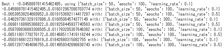
結論:batch:50、epochs:100、学習率:0.1が最も良いことが分かった
活性化関数もパラスタする
| 因子 | 1水準目 | 2水準目 | 3水準目 |
|---|---|---|---|
| 活性化関数 | ReLu | Swish | Mish |
| 学習率 | 0.1 | 0.5 | |
| epochs | 100 | 300 | |
| batchサイズ | 50 | 100 |
# Importing the necessary packages
from sklearn.model_selection import GridSearchCV, KFold
from keras.models import Sequential
from keras.layers import Dense
from keras.losses import mean_squared_error
import tensorflow as tf
from tensorflow.keras.layers import Activation
from tensorflow.keras.utils import get_custom_objects
#分類問題用のライブラリ
#from keras.wrappers.scikit_learn import KerasClassifier
#回帰問題用nライブラリ
from keras.wrappers.scikit_learn import KerasRegressor

from keras.optimizers import Adam
from keras.layers import Dropout
#============================================================================
class Mish(Activation):
    '''
    Mish Activation Function.
    .. math::
        mish(x) = x * tanh(softplus(x)) = x * tanh(ln(1 + e^{x}))
    Shape:
        - Input: Arbitrary. Use the keyword argument `input_shape`
        (tuple of integers, does not include the samples axis)
        when using this layer as the first layer in a model.
        - Output: Same shape as the input.
    Examples:
        >>> X = Activation('Mish', name="conv1_act")(X_input)
    '''

    def __init__(self, activation, **kwargs):
        super(Mish, self).__init__(activation, **kwargs)
        self.__name__ = 'Mish'
def mish(inputs):
    return inputs * tf.math.tanh(tf.math.softplus(inputs))
get_custom_objects().update({'Mish': Mish(mish)})
#============================================================================
# DNNモデル定義
def create_model(learning_rate,active):
    model = Sequential()
    model.add(Dense(64,input_dim = 8,kernel_initializer = 'normal',activation = active))
    model.add(Dense(32,activation = active))
    model.add(Dense(16,activation = active))
    model.add(Dense(8,activation = active))
    model.add(Dense(1,activation = 'linear'))

    adam = Adam(lr = learning_rate)
    #model.compile(loss = 'binary_crossentropy',optimizer = adam,metrics = ['acc'])
    model.compile(loss = 'mse',optimizer = adam,metrics = ['mae'])
    return model

# Create the model
#model = KerasClassifier(build_fn = create_model,verbose = 0,batch_size = 40,epochs = 10)

# Define the grid search parameters
active=['relu','swish','Mish']
epochs_grid=[100,300]
batch_size_grid=[50,100]
learning_rate = [0.1,0.5]

### the grid search parametersを辞書型で定義する
param_grids = dict(active=active,learning_rate = learning_rate,batch_size=batch_size_grid,epochs=epochs_grid)
#分類問題の設定
#model = KerasClassifier(build_fn = create_model,verbose = 0,batch_size = batch_size_grid,epochs = epochs_grid)
#回帰問題の設定
model=KerasRegressor(build_fn=create_model,verbose=0,batch_size = batch_size_grid,epochs = epochs_grid)
# Build and fit the GridSearchCV

grid = GridSearchCV(estimator = model,param_grid = param_grids,cv = KFold(),verbose = 1)
grid_result = grid.fit(x_train,y_train)

# 結果のまとめを表示

print('Best : {}, using {}'.format(grid_result.best_score_,grid_result.best_params_))
means = grid_result.cv_results_['mean_test_score']
stds = grid_result.cv_results_['std_test_score']
params = grid_result.cv_results_['params']
for mean, stdev, param in zip(means, stds, params):
    print('{},{} with: {}'.format(mean, stdev, param))
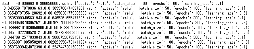
結論:活性化関数:ReLU、batch:100、epochs:100、学習率:0.1が最も良いことが分かった
ニューロン数もパラスタする
| 因子 | 1水準目 | 2水準目 | 3水準目 |
|---|---|---|---|
| 活性化関数 | ReLu | ||
| 学習率 | 0.1 | ||
| epochs | 100 | ||
| batchサイズ | 100 | ||
| 1層目のニューロン数 | 64 | 128 | 256 |
※2層目は1層目のニューロン数の50%、3層目は1層目の25%・・・としていく
# Importing the necessary packages
from sklearn.model_selection import GridSearchCV, KFold
from keras.models import Sequential
from keras.layers import Dense
from keras.losses import mean_squared_error
import tensorflow as tf
from tensorflow.keras.layers import Activation
from tensorflow.keras.utils import get_custom_objects
#分類問題用のライブラリ
#from keras.wrappers.scikit_learn import KerasClassifier
#回帰問題用nライブラリ
from keras.wrappers.scikit_learn import KerasRegressor

from keras.optimizers import Adam
from keras.layers import Dropout

#============================================================================
class Mish(Activation):
    '''
    Mish Activation Function.
    .. math::
        mish(x) = x * tanh(softplus(x)) = x * tanh(ln(1 + e^{x}))
    Shape:
        - Input: Arbitrary. Use the keyword argument `input_shape`
        (tuple of integers, does not include the samples axis)
        when using this layer as the first layer in a model.
        - Output: Same shape as the input.
    Examples:
        >>> X = Activation('Mish', name="conv1_act")(X_input)
    '''

    def __init__(self, activation, **kwargs):
        super(Mish, self).__init__(activation, **kwargs)
        self.__name__ = 'Mish'
def mish(inputs):
    return inputs * tf.math.tanh(tf.math.softplus(inputs))
get_custom_objects().update({'Mish': Mish(mish)})
#============================================================================

# DNNモデル定義
def create_model(learning_rate,active,neuron):
    model = Sequential()
    #ポイント:float型に変更
    neuron=float(neuron)
    neuron2=int(neuron/2)
    neuron3=int(neuron/4)
    neuron4=int(neuron/8)
    #最後にint型に戻す
    neuron=int(neuron)
    model.add(Dense(neuron,input_dim = 8,kernel_initializer = 'normal',activation = active))
    model.add(Dense(neuron2,activation = active))
    model.add(Dense(neuron3,activation = active))
    model.add(Dense(neuron4,activation = active))
    model.add(Dense(1,activation = 'linear'))

    adam = Adam(lr = learning_rate)
    #model.compile(loss = 'binary_crossentropy',optimizer = adam,metrics = ['acc'])
    model.compile(loss = 'mse',optimizer = adam,metrics = ['mae'])
    return model

# Create the model
#model = KerasClassifier(build_fn = create_model,verbose = 0,batch_size = 40,epochs = 10)

# Define the grid search parameters
active=['relu']
epochs_grid=[100]
batch_size_grid=[100]
learning_rate = [0.1]
neuron=['64','128','256']

### the grid search parametersを辞書型で定義する
param_grids = dict(active=active,neuron=neuron,learning_rate = learning_rate,batch_size=batch_size_grid,epochs=epochs_grid)
#回帰問題の設定
model=KerasRegressor(build_fn=create_model,verbose=0,batch_size = batch_size_grid,epochs = epochs_grid)
# Build and fit the GridSearchCV
grid = GridSearchCV(estimator = model,param_grid = param_grids,cv = KFold(),verbose = 1)
grid_result = grid.fit(x_train,y_train)

# 結果のまとめを表示
print('Best : {}, using {}'.format(grid_result.best_score_,grid_result.best_params_))
means = grid_result.cv_results_['mean_test_score']
stds = grid_result.cv_results_['std_test_score']
params = grid_result.cv_results_['params']
for mean, stdev, param in zip(means, stds, params):
    print('{},{} with: {}'.format(mean, stdev, param))

結論:ニューロン数はINPUT8→64→32→16→8→OUT:1が最も良いことが分かったことが分かった
まとめ
GridSearchは全数探査なので、計算コストは増加する。
しかし、人間が調整する手間を省けるので、有効活用できそうだ。
直交実験計画をうまく組み込めたらもっと少ない検討数で探査できそうなので
また考えてみようと思う。
以上 最後までお読みいただきありがとうございました。