BayesAssによる移入率の推定
BayesAssで集団ごとの移入率の推定を行うにあたり、混合パラメーターの探索が面倒であるのと、探索の結果得られた混合パラメーターが適切であるかわからないので腰が重かった。
テストラン的にパラメーターの推定を行ってくれるBA3-SNPS-autotuneなるものを発見したので、試しに使ってみました。
解析の流れとして、
-
BA3-SNPS-autotuneによるパラメーターの推定→収束確認 -
BayesAssによる本解析→収束確認
という流れになりそう。
BA3-SNPSとBA3-SNPS-autotuneの両方が安全に動かせるDocker仮想環境BayesAss3-SNPsが公開されているので、これを導入、解析、可視化するとこまでをメモがてら書いていきます。
間違っていたら教えてください。
導入
実行環境
- Windows 11
- Ubuntu 22.04
- Docker
0. Dockerの導入
Docker Engine導入する場合(Linux, WSL)
Docker Desktopを使用する場合は不要です。
参考:https://matsuand.github.io/docs.docker.jp.onthefly/engine/install/ubuntu/
手順通りinstall
sudo apt-get remove docker docker-engine docker.io containerd runc
sudo apt-get update
 sudo apt-get install \
    ca-certificates \
    curl \
    gnupg \
    lsb-release
echo \
  "deb [arch=$(dpkg --print-architecture) signed-by=/usr/share/keyrings/docker-archive-keyring.gpg] https://download.docker.com/linux/ubuntu \
  $(lsb_release -cs) stable" | sudo tee /etc/apt/sources.list.d/docker.list > /dev/null
curl -fsSL https://download.docker.com/linux/ubuntu/gpg | sudo gpg --dearmor -o /usr/share/keyrings/docker-archive-keyring.gpg
 sudo apt-get update
 sudo apt-get install docker-ce docker-ce-cli containerd.io docker-compose-plugin
Dockerのinstallに成功しているか確認
$ sudo docker run hello-world
Unable to find image 'hello-world:latest' locally
latest: Pulling from library/hello-world
e6590344b1a5: Pull complete
Digest: sha256:7e1a4e2d11e2ac7a8c3f768d4166c2defeb09d2a750b010412b6ea13de1efb19
Status: Downloaded newer image for hello-world:latest

Hello from Docker!
This message shows that your installation appears to be working correctly.

To generate this message, Docker took the following steps:
 1. The Docker client contacted the Docker daemon.
 2. The Docker daemon pulled the "hello-world" image from the Docker Hub.
    (amd64)
 3. The Docker daemon created a new container from that image which runs the
    executable that produces the output you are currently reading.
 4. The Docker daemon streamed that output to the Docker client, which sent it
    to your terminal.

To try something more ambitious, you can run an Ubuntu container with:
 $ docker run -it ubuntu bash

Share images, automate workflows, and more with a free Docker ID:
 https://hub.docker.com/

For more examples and ideas, visit:
 https://docs.docker.com/get-started/
こうなっていれば大丈夫そうです。
dockerコマンド実行時にsudoが必要だと、./buildDocker.shが実行失敗するので、
Got permission denied while trying to connect to the Docker daemon socket at unix:///var/run/docker.sock: Get "http://%2Fvar%2Frun%2Fdocker.sock/v1.24/containers/json": dial unix /var/run/docker.sock: connect: permission denied
sudoなしでdockerコマンドを実行できるようにする。
dockerに指示を出す際に経由されるsocketファイルにsuper user権限を付与します。
sudo chmod 666 /var/run/docker.sock
sudoなしのdockerコマンドでエラーが出てこなければ大丈夫です。
docker ps
CONTAINER ID   IMAGE     COMMAND   CREATED   STATUS    PORTS     NAMES
1. リポジトリをclone
git clone https://github.com/stevemussmann/BayesAss3-SNPs.git
一応、ソースコードを直接DLしても以下は同じ方法でいけると思います。
2. Docker環境構築
# 環境構築用スクリプトがあるディレクトリに移動
cd /hoge/huga/BayesAss3-SNPs/Docker

# 仮想環境をbuild
./buildDocker.sh
3. 仮想環境の起動
$ ./runDocker.sh
You can copy your data for ba3snps into this directory and
it will be accessible at "/app/data" in the Docker container.


Starting docker container for mussmann/ba3snps.

Type "exit" at the command prompt to exit the container.
Only data saved in "/app/data" will be retrievable after exiting.
All data saved in other locations within the container will
be lost upon exiting.


ba3user@0a5644a57093:/app/data$
このようになれば導入はおおよそ成功です。
おそらく、Dockerディレクトリ内にdataディレクトリが作成されているはずです。
dataディレクトリは、入力ファイル置き場で、このディレクトリに入っているファイルは仮想環境内からもアクセス可能になるみたいです(Volumeマウントしていると思います)。
# 確認
hoge:/hoge/huga/BayesAss3-SNPs/Docker$ ls
Dockerfile  buildDocker.sh  data  runDocker.sh
以下、構築した環境内で実行していきます。
BayesAss解析
1. BA3-SNPS-autotuneによるパラメーターの推定
事前にSNPデータをBayeAssのインプット形式に変換しておきます(PGDSpiderあたり?)。
※このとき集団(population)の設定を行う(しなくても実行可能だと思われるが、集団=個体としていると、個体ごとの移入(意味不明)が推定されそうなので)。
dataディレクトリに入力ファイルを移動しておきます。
# BA3-SNPS-autotuneの実行
ba3user@0a5644a57093:/app$ ./bin/BA3-SNPS-autotune.py -i ./data/vcf_cut_u108_pop_all.recode.bayesass.txt -o test_test -l 140
78 -g 500000 -b 50000
MCMCの値は数百万回をよく見ますが、自分の場合は数億回指定してやっと収束しました...
burn-inはMCMCの10%を目安にtraceファイルを確認しながら調整するのがよさそうです。
-
Tracerで確認
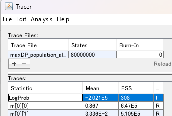
ESEの値がすべて200を超えていれば収束とみなしてよさそうです。
EstimatesやMarginal Density、Traceも確認してMCMC chainが正常に収束しているか確認します。
BEASTのトラブルシューティングですが、Tracerの収束確認はこちらを参照するとよいかも?
-
混合パラメータ値の確認
*.finalParams.txtというファイルにautotuneで推定された混合パラメータ値が書きこまれています。*.finalParams.txt##Tuning completed early after 4 rounds. ##M A F 0.3 0.8 0.03収束を確認したら、
BA3-SNPSのパラメータに代入するため、控えておきます。
こちらの値はそれぞれBA3の同名のオプションの引数として代入します。# -m --deltaM 移住率の混合パラメータ値(0<ΔM≤1.0) # -a --deltaA 対立遺伝子頻度の混合パラメータ値(0<ΔA≤1.0) # -f --deltaF 近交係数の混合パラメータ値(0<ΔF≤1.0)基本的にautotuneで出た値を使えば、MCMCの
acceptedの値は適切になりそうです。
2. BA3-SNPSの実行
上記Dockerコンテナ内でBA3-SNPSを同時に実行できればよかったのですが、出力ファイルがどこに吐き出されているか不明だったので、autotuneと統合前のBA3から実行しています。
M → -m、A → -a、F → -fのように置き換えて代入
BA3SNP -v -t -g -i 500000 -n 50000 -n 5000 -m 0.3 -a 0.8 -f 0.03 ./data/tetest_data.recode.bayesass.txt
結果の見方についてはこちらの記事やBA3のマニュアルを参照ください。
Tracerで、autotuneと同様に収束していればOK
以下、個人的メモです
採択率について
The acceptance rates for proposed changes to parameters 1, 3 and 4 in the above list (migration rates, allele frequencies and inbreeding coefficients, respectively) can be adjusted by changing the values of the respective mixing parameters. If the acceptance rate is too high, the chain does not mix well, often proposing values very near the current value (which are accepted) and failing to adequately explore the state space. If the acceptance rate is too low the chain rarely accepts the proposed moves which are too different from the current value – this also causes poor mixing. Empirical analyses suggest that an acceptance rate between 20% and 60% is optimal.
migration rates, inbreeding coefficients, respectivelyのacceptedの値が20-60%の範囲に入るとよさそうです
95%信頼区間の出し方
95%信頼区間は直接出力されないですが、計算で大まかに出せるみたいです。
A rough 95% credible set can be constructed as mean ± 1.96 × sdev.
例えば、
m[0][0]: 0.540(0.0100)
上記の場合、0.540 ± 1.96 × 0.010 = ± 0.025となり、信頼区間と中央値は0.540[0.515-0.565]ということでしょうか。
あまりBayessAssを利用している論文で、言及されていないことが多いのですが、以下のような値も出ます。
# 各集団の近郊係数(Inbreeding Coefficients)のFstおよび事後確率(標準誤差)
 Inbreeding Coefficients:

HP Fstat: 0.1101(0.0060)
OP Fstat: 0.0918(0.0052)
YP Fstat: 0.1053(0.0056)
CP Fstat: 0.0528(0.0063)
CMP Fstat: 0.0736(0.0053)

# 集団と座位ごとの対立遺伝子頻度
Allele Frequencies:

HP
4:73>>
4:0.667(0.130) 1:0.333(0.130)
22:1>>
1:0.577(0.141) 4:0.423(0.141)
23:78>>
3:0.820(0.108) 2:0.180(0.108)
結果の可視化
流れとしては、「移入率データの成形→Rで可視化」です。
こちらを参考に、所謂Chord diagramを生成していきます。
1. データの成形
*out.txtに欲しいデータが入っているので、エクセルなどでCSVやTXT形式に書き起こす。(例では元データの標準偏差は省いて書いています)
[i][j]は集団i→集団jの移入率です。
# *out.txtの元データ
Migration Rates:

 m[0][0]: 0.5000 m[0][1]: 0.1000 m[0][2]: 0.1000 m[0][3]: 0.1000 m[0][4]: 0.1000 m[0][5]: 0.1000
 m[1][0]: 0.6000 m[1][1]: 0.2000 m[1][2]: 0.1000 m[1][3]: 0.0500 m[1][4]: 0.0400 m[1][5]: 0.0100
 m[2][0]: 0.4000 m[2][1]: 0.5000 m[2][2]: 0.0500 m[2][3]: 0.0300 m[2][4]: 0.0100 m[2][5]: 0.0100
 m[3][0]: 0.9000 m[3][1]: 0.0200 m[3][2]: 0.0200 m[3][3]: 0.0.0200 m[3][4]: 0.0200 m[3][5]: 0.0200
 m[4][0]: 0.3000 m[4][1]: 0.3000 m[4][2]: 0.1500 m[4][3]: 0.0200 m[4][4]: 0.1000 m[4][5]: 0.1200
 m[5][0]: 0.0200 m[5][1]: 0.0300 m[5][2]: 0.0200 m[5][3]: 0.0300 m[5][4]: 0.1000 m[5][5]: 0.8000

↓

# CSV
# 以降、migratoin_rate.csv
0,1,2,3,4,5
0.5000,0.1000,0.1000,0.1000,0.1000,0.1000
0.6000,0.2000,0.1000,0.0500,0.0400,0.0100
0.4000,0.5000,0.0500,0.0300,0.0100,0.0100
0.9000,0.0200,0.0200,0.0200,0.0200,0.0200
0.3000,0.3000,0.1500,0.2000,0.1000,0.1200
0.0200,0.0300,0.0200,0.0300,0.1000,0.8000
以下、Rで作業していきます。
# データの読み込み
data <- read.table("migration_rate.csv", header = TRUE, sep = ",", quote = "\"", dec = ".", fill = TRUE, comment.char = "")
# 行データの名前変更
colnames(data) <- c("A","B","C","D","E","F")
# 列データの名前変更
rownames(data) <- colnames(data)
順番を間違えないように注意してください。総当たり表みたいになっていればひとまず大丈夫です。
2. 図表のパラメータ設定
# 必要なlibrary
library(tidyverse)
library(hrbrthemes)
library(circlize)
library(kableExtra)
options(knitr.table.format = "html")
library(viridis)
library(igraph)
library(ggraph)
library(colormap)
この辺はまだよくわかっていないのでコピペしてます。
# I need a long format
data_long <- data %>%
  rownames_to_column %>%
  gather(key = 'key', value = 'value', -rowname)

# parameters
circos.clear()
circos.par(start.degree = 90, gap.degree = 4, track.margin = c(-0.1, 0.1), points.overflow.warning = FALSE)
par(mar = rep(0, 4))
色の設定
ほぼコピペですがデータ数に合わせて数値変更します。
# color palette
mycolor <- viridis(6, alpha = 1, begin = 0, end = 1, option = "D")
mycolor <- mycolor[sample(1:6)]
今回は6集団なので、6色になるように設定していきます。
このままコピペすると集団の数にあわせてカラーセットから割り当てるようになっていますので、適宜色は指定してください。
chordDiagramのパラメーター設定
# Base plot
chordDiagram(
  x = data_long,
  grid.col = mycolor,
  transparency = 0.25,
  directional = 1,
  direction.type = c("arrows", "diffHeight"),
  diffHeight  = -0.04,
  annotationTrack = "grid",
  annotationTrackHeight = c(0.05, 0.1),
  link.arr.type = "big.arrow",
  link.sort = TRUE,
  link.largest.ontop = TRUE)
この辺もコピペです。
# Add text and axis
circos.trackPlotRegion(
  track.index = 1,
  bg.border = NA,
  panel.fun = function(x, y) {

    xlim = get.cell.meta.data("xlim")
    sector.index = get.cell.meta.data("sector.index")

    # Add names to the sector.
    circos.text(
      x = mean(xlim),
      y = 3.2,
      labels = sector.index,
      facing = "bending",
      cex = 0.8
      )

    # Add graduation on axis
    circos.axis(
      h = "top",
      major.at = seq(from = 0, to = xlim[2], by = ifelse(test = xlim[2]>10, yes = 2, no = 1)),
      minor.ticks = 1,
      major.tick.percentage = 0.5,
      labels.niceFacing = FALSE)
  }
)
`major.tick.percentage` is not used any more, please directly use argument `major.tick.length`.
完成
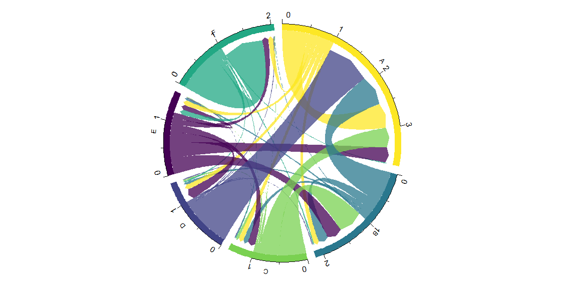
バーの数値と地点名が重複していますが、適宜調整してください...
↑の場合、0-1の範囲から出ている帯はその集団から移住する個体の総量で、1-2の範囲には他の集団から入ってくる個体を示しています。
もう少しいい可視化方法あったら教えてください。
参考
BayesAss関連
- BA3-SNPS-autotune: Mussmann, S. M., Douglas, M. R., Chafin, T. K., & Douglas, M. E. (2019). BA3‐SNPs: Contemporary migration reconfigured in BayesAss for next‐generation sequence data. Methods in Ecology and Evolution, 10(10), 1808-1813. https://doi.org/10.1111/2041-210X.13252
- BayesAssを用いた最近の移住率の推定 @YF_bio