

はじめに
SS 433を扱っていると、ある瞬間に何がどこにあって、どちらを向いているのかをイメージしにくい場面がかなりあります。
代表的なものだけでも、
- 約13日のbinary orbit
- 約162日のjet precession
- 約6.3日のnutation / nodding
という複数の周期があります。
さらに、jet sourceであるcompact object自身が公転しており、そこから放出されたjet materialは約$0.26c$で外側へ進みます。arcsec scaleに見えているjetは、その瞬間のjet axisそのものではなく、過去の異なるphaseで放出されたmaterialの履歴です。
個々の要素については、これまで少しずつ整理してきました。
- SS 433の三次元歳差モデルを数式で理解する:幾何と座標変換の整理
- SS 433の歳差ジェットを空に投影する:光の到達時間効果をPythonで可視化する
- SS 433のノッディング周期を Katz et al. (1982) からたどる:理論と観測の間で
ただ、それぞれを別々に見ても、binary orbit、precession、nutation、ballistic propagationを頭の中で同時に動かすのはなかなか大変です。
そこで今回は、これまで調べてきた範囲を一つのkinematic modelにまとめ、SS 433の全体的なgeometryを一度に眺められるanimationを作ってみました。
目的は精密なsimulationではなく、
SS 433では、どのような運動が、どの程度のscaleで、同時に重なっているのか
を直感的に見ることです。
最初に:これは説明用のtoy modelです
今回作るのはkinematic toy modelです。
binary evolutionやaccretion diskのhydrodynamicsを解いているわけではありません。
一方で、単なる模式図として好きな大きさ・速度で動かすのではなく、
- binary separation
- componentのbarycentric orbit
- jet speed
- precession geometry
- distance
- light-travel-time effect
などについては、可能な範囲でphysical scaleを保つようにしています。
したがって、
physical scaleを保った可視化ではありますが、physical simulationではありません。
特に、
- component mass
- disk geometry
- companionの形状
- nutationの三次元的な表現
などにはmodel assumptionがあります。
今回のanimationを実データへそのままfitしたり、ここから定量的なsystem parameterを決めたりする用途は想定していません。
以下では、今回のmodelに何を入れたのかを順番に整理します。
今回使うparameter set
基本的なkinematic parametersには、Roberts et al. (2010)にまとめられているephemerisを主に参考にしました。
| parameter | value |
|---|---|
| orbital period, $P_{\rm orb}$ | 13.08211 d |
| precession period, $P_{\rm prec}$ | 162.375 d |
| jet speed, $\beta=v/c$ | 0.2647 |
| precession half-opening angle | $20.92^\circ$ |
| inclination | $78.05^\circ$ |
| position angle | $98.2^\circ$ |
| nutation period | 6.2877 d |
| nutation amplitude in moving-line ephemeris | $z_{\rm nut}=0.009$ |
| adopted tangent-plane wobble radius | $2.0^\circ$ |
| distance | 5.5 kpc |
kinematic parametersには文献やephemerisによって多少の違いがあります。
以前の記事では、$P_{\rm prec}=162.15$ d、$\beta=0.2602$、$i=78.83^\circ$、$\theta=19.85^\circ$など、別のparameter setも使っています。
今回はparameter estimationが目的ではないため、一つのまとまったsetとしてRoberts et al. (2010)側の値を採用しました。
1. 約13日のbinary orbit
まずcompact objectとcompanionを、共通重心のまわりの円軌道として動かします。
orbital phaseは、
\phi_{\rm orb}(t)
=
2\pi
\frac{t-t_{\rm orb,0}}{P_{\rm orb}}
です。
binary separationを$a$、compact objectとcompanionの質量をそれぞれ$M_{\rm c}$、$M_{\rm d}$とすると、
r_{\rm c}
=
a\frac{M_{\rm d}}{M_{\rm c}+M_{\rm d}},
\qquad
r_{\rm d}
=
a\frac{M_{\rm c}}{M_{\rm c}+M_{\rm d}}
としてbarycenterまわりの軌道半径を決めます。
したがって、
M_{\rm d}\mathbf r_{\rm d}
+
M_{\rm c}\mathbf r_{\rm c}
=
0
が常に成り立ちます。
component massについては現在もmodel dependenceが大きいため、今回は代表値として、
M_{\rm compact}=6\,M_\odot,
\qquad
M_{\rm companion}=12\,M_\odot
を置いています。
これは質量を決定するための値ではありません。
この質量と$P_{\rm orb}$からKeplerの法則でbinary separationを求め、そのscaleをそのままanimationへ使っています。
orbital phase 0はRoberts et al. (2010)のephemerisに合わせ、primary eclipse、つまりcompanionがcompact objectより手前に来るconfigurationとしています。
2. companionはRoche-equivalent sphereとして描く
companionの大きさも、単純に見やすい半径を置くのではなく、Eggleton (1983)のRoche-lobe volume-equivalent radiusを使っています。
ここではdonor / companion側のRoche lobeを求めるので、質量比を明示的に
q_{\rm d}\equiv
\frac{M_{\rm companion}}{M_{\rm compact}}
と定義します。Eggletonの式は、
\frac{R_{\rm L}}{a}
=
\frac{
0.49q^{2/3}
}{
0.6q^{2/3}
+
\ln(1+q^{1/3})
}
です。
今回の値では$q_{\rm d}=12/6=2$です。SS 433の文献でよく使われる
$q=M_{\rm compact}/M_{\rm companion}$とは逆数なので、コード側でも
Q_DONOR_OVER_COMPACTという名前にしています。
ただし、描いているのはこの半径を持つ球です。
実際のRoche surfaceそのものではありません。
したがって、animationの中央panelで、
- companionとcompact objectのどちらが手前か
- compact objectの中心がcompanionの投影内へ入っているか
を見ることはできますが、精密なeclipse modelではありません。
mass-transfer streamなども入れていません。
3. 約162日のretrograde precession
jet axisは、平均軸のまわりを約162日でprecessionさせます。
binary frameを右手系$(X_b,Y_b,Z_b)$として、
+\hat{\mathbf Z}_b
=
+\hat{\mathbf L}_{\rm orb}
と置きます。
precession coneのhalf-opening angleを$\theta_{\rm p}$、precession phaseを$\phi_{\rm p}$とすると、
\mathbf n_{\rm prec}(t)
=
\begin{pmatrix}
\sin\theta_{\rm p}\cos\phi_{\rm p}(t)\\
\sin\theta_{\rm p}\sin\phi_{\rm p}(t)\\
\cos\theta_{\rm p}
\end{pmatrix}
です。
今回のmodelでは、
\phi_{\rm p}(t)
=
-2\pi
\frac{t-t_{\rm prec,0}}{P_{\rm prec}}
として、binary orbitに対してretrogradeなprecessionを採用します。
コードでは、
ORBIT_SENSE = +1
PREC_SENSE = -1
です。
precessionを逆向きにする根拠
SS 433のstandard kinematic modelでは、Hjellming & Johnston (1981)以来、jet precessionのrotation-sense parameterとして$s=-1$が使われています。
またdynamicalな解釈として、Collins & Scher (2002)ではprecessing objectについてorbital motionに対するretrograde precessionを扱い、precession angular frequencyを負として定義しています。
したがって今回のmodelでは、
\boldsymbol{\omega}_{\rm orb}\cdot\mathbf L_{\rm orb}>0
に対して、
\boldsymbol{\omega}_{\rm prec}\cdot\mathbf L_{\rm orb}<0
となるgeometryを採用しました。
これは画面上で単純に「時計回り/反時計回り」と決めているのではなく、angular-velocity vectorの符号で定義しています。
precession geometry自体については、以前の記事で詳しく整理しています。
SS 433の三次元歳差モデルを数式で理解する:幾何と座標変換の整理
4. 約6日のnutation / nodding
さらに、約162日のprecessionに加えて、より短周期のnutation / noddingも重ねています。
SS 433では、moving-line velocityやdisk orientationに約6日程度の短周期変動が見られることが古くから知られています。Katz et al. (1982)では、この変動を、binary companionから時間依存のtidal torqueを受けるprecessing accretion ring / diskのnoddingとして説明するmodelが議論されました。その後も、diskの構造や内部回転、外力の扱いなどを変えた複数のdynamical modelが検討されています。
一方で、観測される約6日の周期やredshift変動から、disk normalやjet axisが三次元空間で描くtrajectoryを一意に決められるわけではありません。
したがって今回は、
約6日のnoddingという観測的・理論的特徴と、その運動をanimation上でどのような三次元trajectoryとして表現するかは分けて考える
ことにします。
以下では、文献で議論されているcone angleとprecessional phaseの短周期変動を参考にしつつ、説明用のkinematic prescriptionとしてnutationを実装します。
Collins & Scher (2002)では、jet orientationを記述する2つの角度、すなわちprecession cone angleとprecessional phaseにsmall-amplitudeのsinusoidal oscillationを加える形でnodding motionを表しています。そこで今回のanimationでも、このdouble-angularな表現を参考に、
\theta(t)
=
\theta_{\rm p}
+
\delta\theta_{\rm nut}(t)
\phi(t)
=
\phi_{\rm p}(t)
+
\delta\phi_{\rm nut}(t)
とします。
それぞれを単純なsinusoidal componentとして、
\delta\theta_{\rm nut}(t)
=
A_\theta
\sin
\left[
2\pi
\frac{t-t_{\rm nut,0}}{P_{\rm nut}}
+
\varphi_\theta
\right]
\delta\phi_{\rm nut}(t)
=
A_\phi
\sin
\left[
2\pi
\frac{t-t_{\rm nut,0}}{P_{\rm nut}}
+
\varphi_\phi
\right]
としています。
最終的なlaunch directionは、
\mathbf n(t)
=
\begin{pmatrix}
\sin\theta(t)\cos\phi(t)\\
\sin\theta(t)\sin\phi(t)\\
\cos\theta(t)
\end{pmatrix}
です。
ここで重要なのは、この具体的な三次元wobbleは今回のtoy-model prescriptionだという点です。
約6日のnodding自体には観測・理論的な背景がありますが、今回の$\delta\theta$と$\delta\phi$の組み合わせがSS 433のdisk dynamicsを一意に表しているわけではありません。
6.06日と6.29日
ここは「理論周期」と「観測ephemeris」を同じものとして扱わないことが重要です。
retrograde precessionの大きさを正の周波数$f_{\rm prec}=1/P_{\rm prec}$で書くと、
Katz et al. (1982)のdouble-angular motionの基本周波数は、
f_{\rm hs}=2(f_{\rm orb}+f_{\rm prec})
で、対応するhalf-synodic periodは今回のparameterでは
$P_{\rm hs}=6.05335$ d、丸めて約6.06 dです。
ただし、cone angleとprecessional phaseのこの基本振動をstandard redshift equationへ通すと、
precession周波数だけ離れた成分が現れます。
f_{\rm long}=f_{\rm hs}-f_{\rm prec},
\qquad
f_{\rm short}=f_{\rm hs}+f_{\rm prec}.
今回のparameterでは、
P_{\rm long}=6.28776\ {\rm d},
\qquad
P_{\rm short}=5.83579\ {\rm d}
となります。Katz et al. (1982)では、moving-lineの$z$ residualで約6.28 dが卓越し、
約5.83 dも検出される一方、理想化したmodelでは中心の約6.06 d成分が相殺されることが示されています。
したがって、約6.29 dは約6.06 dと無関係な別時計ではなく、precession geometryを通して現れるsidebandとして理解できます。
Roberts et al. (2010)のradio-locus ephemerisでは、観測的なdominant termとして
P_{\rm nut}=6.2877\ {\rm d}
が使われています。animationのdefaultもこの値を維持します。ただし現在のanimationは
single-periodのangular wobbleとして実装しており、6.06/6.29/5.84 dの全spectral structureを
同時に再現するdynamical modelではありません。
この違いについては、以前の記事で少し詳しく追っています。
SS 433のノッディング周期を Katz et al. (1982) からたどる:理論と観測の間で
nutationのangular prescription
Roberts et al. (2010)のTable 1にはNutation Amplitude = 0.009とありますが、
単位は明記されていません。同じephemerisを説明するMarshall et al. (2013)では、
この量が明示的に
z_{\rm nut}=0.009
と書かれています。したがって、0.009をradと解釈して角度へ直接変換することはしません。
standard kinematic redshiftを
z_\pm=\gamma(1\mp\beta\cos\alpha)-1
とすると、小さな方向変化$\delta\alpha$に対して、
|\Delta z|\simeq\gamma\beta\sin\alpha\,|\delta\alpha|
です。$\beta=0.2647$でLOS感度が最大の$\sin\alpha=1$なら、
$|\Delta z|=0.009$に相当する角度は$1.88^\circ$です。標準geometryでは
$\alpha=57.13^\circ$から$98.97^\circ$の範囲なので、今回は丸めた
A_{\rm tangent}=2.0^\circ
をtangent-plane上の代表的なwobble radiusとして採用します。これはmoving-line dataへのfitではなく、
$z_{\rm nut}$とorder-of-magnitudeで整合するように導いたscaleです。Fabrika (2004)などで引用される
約$2.8^\circ$のnodding angleとも同じ「数度」の範囲ですが、定義が同一とは限らないため、
その$2.8^\circ$をコードへ直接代入してはいません。
double-angular representationでは、
A_\theta=2.0^\circ
とし、$\phi$方向のtangent lengthが同じになるよう、
\sin\theta_{\rm p}\,A_\phi=A_{\rm tangent}
から$A_\phi=5.60^\circ$とします。2成分はquadratureに置きます。
ここで、$\sin\theta_{\rm p}A_\phi\simeq A_\theta$としてunit sphere上でほぼ円形のwobbleを作ること、
2成分の位相差、handedness、観測ephemerisのzero pointを各角度成分へ割り当てる方法は、
すべて今回のvisualization prescriptionです。Collins & Scher (2002)が支持するのは
cone angleとprecessional phaseのsmall sinusoidal oscillationという構造であり、この円軌道そのものではありません。
nutation parameterの由来
| parameter | value | classification |
|---|---|---|
| observed period | 6.2877 d | literature value / observational ephemeris |
| observed reference epoch | JD 2450000.94 | literature value / observational ephemeris |
| moving-line amplitude | $z_{\rm nut}=0.009$ | literature value |
| half-synodic fundamental | 6.05335 d | derived value |
| long / short sidebands | 6.28776 / 5.83579 d | derived value |
| maximum-sensitivity equivalent angle | $1.88^\circ$ | derived value |
| adopted tangent wobble radius | $2.0^\circ$ | derived value(rounded) |
| $A_\theta$ | $2.0^\circ$ | toy-model assumption |
| $A_\phi$ | $5.60^\circ$ | toy-model assumption |
| quadrature phase / handedness | $\varphi_\theta=\pi/2,\ \varphi_\phi=0$ | toy-model assumption |
| literature comparison angle | about $2.8^\circ$ | literature value; not adopted directly |
この処方をstandard redshift equationで数値確認すると、precession phaseごとの
$\Delta z$ semi-amplitudeは0.00805–0.00958、medianは0.00942、全phaseをまとめた
equivalent sinusoidal amplitudeは0.00910です。したがって観測的な$z_{\rm nut}\sim0.009$と
整合する代表scaleですが、厳密fitではありません。
5. diskはjet directionに垂直な薄い円盤として置く
中心部には、jet directionをnormalとする薄いcircular diskも表示しています。
今回は半径を約$8,R_\odot$とし、不透明なdiskとして描いています。
この$8,R_\odot$はouter diskについてのliterature-motivated representative scaleです。
今回仮定した$M_{\rm compact}=6,M_\odot$、$M_{\rm companion}=12,M_\odot$から
自己無撞着に決めたdisk radiusではなく、精密なRoche / accretion-disk modelとしては扱いません。
これは、
- jet / disk axisがどちらを向いているか
- observerから見てdiskのどちら側が手前か
を見やすくするためです。
ただし、
- disk thickness
- disk warpの空間構造
- supercritical disk内部
- wind
などは計算していません。
特にnutationを入れたとき、disk normalもjet directionと完全に一致して動かしていますが、これも今回のkinematic representationです。
6. moving nozzleからjetを放出する
jet sourceであるcompact object自身もbinary orbitを動いています。
したがって、jetは固定された原点からではなく、その時刻のcompact object位置から放出します。
放出時刻を$t_{\rm ej}$とすると、
\mathbf r(t)
=
\mathbf r_{\rm launch}(t_{\rm ej})
+
\mathbf v_{\rm launch}(t_{\rm ej})
(t-t_{\rm ej})
です。
一度放出されたparticleについては、velocityをそのまま固定します。
つまり、放出後のparticleが現在のprecessionやnutationに合わせて曲がるわけではありません。
precessionやnutationによって変化するのは、
各時刻に新しくlaunchされるjet direction
です。
そのため、外側に見える形は、異なる時刻に異なるdirectionで放出されたballistic ejectaの集合になります。
7. compact objectのorbital velocityも加える
launch positionだけでなく、compact object自身のorbital velocityもjetの初速度へ含めています。
$\beta=0.2647$はstandard kinematic parameterとして文献から採用します。ただし、その文献値自体を
「厳密にcompact objectのinstantaneous rest frameで定義された」とまでは主張しません。
今回のコードではmodel assumptionとして、$\beta=0.2647$をcompact-object frameでのlaunch speedと扱い、
compact objectのorbital velocityをspecial-relativistic velocity additionでbarycentric frameへ変換しています。
ただし、
v_{\rm orb}\ll v_{\rm jet}
なので、この効果はlarge-scale morphologyでは小さいものです。
今回の代表質量から得られるcompact objectの公転速度は約158 km s$^{-1}$、
jet speedは約79,355 km s$^{-1}$で、比は$1.99\times10^{-3}$です。
したがってこのframe変換は実装上は保持しますが、arcsec-scale morphologyへの補正は非常に小さいと確認できます。
以前moving-nozzle modelを作ったときにも、binaryのscaleとjetのscaleが大きく異なることを確認しました。
8. jetはballisticに直進する
今回のmodelではjetと周囲物質との相互作用を入れていません。
したがって各ejectaは、launch後に、
- decelerationしない
- deflectionしない
- 周囲のwindに押されない
という理想的なballistic motionです。
これは現実のSS 433 jetを完全に表しているわけではありませんが、precession geometryを見るための基準modelとして使っています。
9. observer座標へ投影する
binary frameから、
- LOS toward Earth
- North
- East
のobserver coordinatesへ変換します。
mean precession axisのsky position angleは$98.2^\circ$としています。
RA-Dec表示では通常の天文画像に合わせてeastが左になるよう、RA axisを反転しています。
distanceには$d=5.5$ kpcを使っています。
Lockman et al. (2007)などでもSS 433の距離として約5.5 kpcが議論されており、今回もこの値を採用しました。
10. light-travel-time effectを入れる
arcsec scaleのjetでは、有限の光速による見かけ位置の違いも入れています。
observer方向を$x$、Earth向きを正とすると、
t_{\rm obs}
=
t_{\rm emit}
-
\frac{x(t_{\rm emit})}{c}
です。
ballistic ejectaではvelocityが一定なので、
\Delta t_{\rm emit}
=
\frac{
t_{\rm obs}-t_{\rm ej}+x_{\rm launch}/c
}{
1-v_x/c
}
と解析的に解くことができます。
そのため見かけ位置は、
\mathbf r_{\rm app}
=
\mathbf r_{\rm launch}
+
\mathbf v\,\Delta t_{\rm emit}
となります。
approaching側とreceding側では、同じobserver timeに見えているejectaのemission ageが異なります。
この部分については以前の記事で詳しく整理しました。
SS 433の歳差ジェットを空に投影する:光の到達時間効果をPythonで可視化する
binaryとjetではscaleが大きく違う
SS 433のjetは約$0.26c$で進みます。
一方、binary separationは0.数AU程度です。
このため、binaryからarcsec jetまでを一つのplot rangeにphysical scaleのまま入れると、中心のbinaryはほとんど一点になります。
今回は物理量そのものを拡大縮小せず、同じmodelを異なるzoomで表示する方法にしました。
明示的なvisualization exaggerationは、
- compact objectのmarker
- instantaneous jet directionを示すfinite guide
だけです。
companion、disk、orbit、ballistic distanceなどは各panel内でphysical scaleを保っています。
animationを見る
MP4(nutation on):https://drive.google.com/file/d/10YpYBu2fjD-8EOgO3LHyg27ZbHFClm9t/view?usp=drive_link
GIF(nutation on):https://drive.google.com/file/d/127FkpmxshIKbHROlcmEs6X_ZQUGgzqxl/view?usp=drive_link
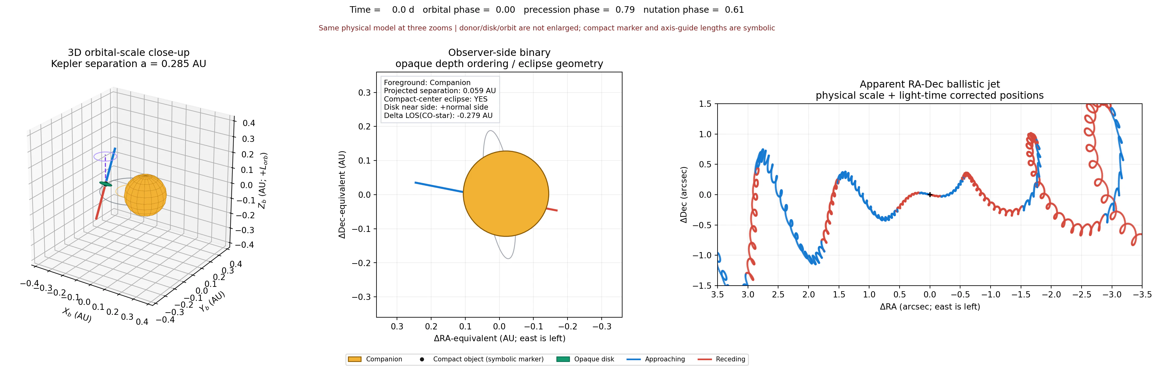
今回のanimationは3 panelです。
左:3D orbital-scale close-up
左はbinary周辺の3D表示です。
- companion
- compact object
- disk
- mean precession cone
- instantaneous approaching / receding direction
を表示しています。
binary orbit、retrograde precession、nutationが同時に動きます。
中央:observer-side binary
中央は同じbinaryをEarth側から見ています。
ここではLOS方向のdepth orderingを使っているため、手前のobjectが上に描かれます。
orbital phase 0付近ではcompanionが手前となり、compact object側を隠します。
約半周期後にはcompact object側が手前になります。
diskもopaqueとしているため、diskのnear / far sideも見やすくしています。
ただし、先ほど述べたように、これは精密なeclipse simulationではありません。
右:RA-Dec ballistic jet
右側では過去に放出されたejectaをRA-Dec上に表示します。
青がapproaching、赤がrecedingです。
各ejection pairについてLOS velocityを比較し、よりEarth向きのbranchをapproachingとしています。
点の大きさは固定です。
今回は約600日分の過去のejectaを保持しています。
\frac{600\ {\rm d}}{162.375\ {\rm d}}
\simeq3.7
なので、約3.7 precession cycle分です。
これによって$\pm3.5$ arcsec程度のfieldまでphysical ballistic ejectaが伸びます。
jet speedやdistanceを表示のために変更しているわけではありません。
nutation ON / OFFを比較する
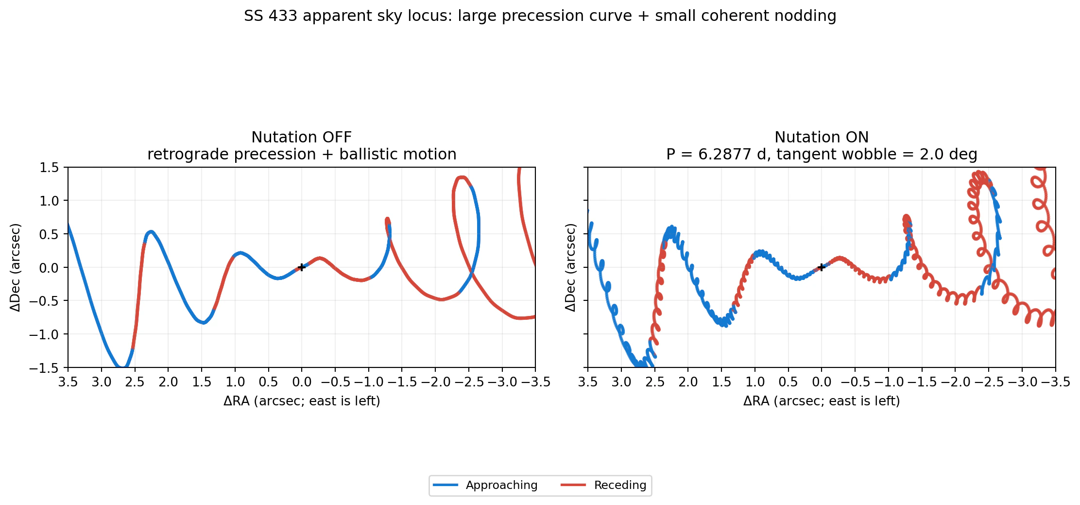
nutationの影響を見るため、同じejection historyについてnutation ON / OFFも比較しています。
左がnutationなし、右がnutationありです。
大局的な形は約162日のprecessionによって決まるため、両者はかなり似ています。
その上に、今回与えた小さなnutationによるwiggleが重なります。
defaultではnutation amplitudeに表示用の倍率を掛けていません。外側ほどwiggleが大きく見えるのは、
同じangular offsetが長いballistic travel distanceで大きなsky displacementになるためです。
この図はnutationの物理modelを検証するためではなく、
precessionによる大きな軌跡に対して、小さな短周期運動を加えるとどの程度の違いになるか
を見るためのものです。
今回入れていないもの
今回のmodelには、少なくとも以下は入っていません。
- eccentric orbit
- detailed Roche surface
- mass-transfer stream
- disk warp dynamics
- supercritical disk structure
- disk wind
- jet launching physics
- jet deceleration
- jet deflection
- jet / ambient-medium interaction
- radiative transfer
- brightness evolution
したがって、右panelもradio imageを再現するmodelではありません。
あくまでkinematic locusです。
数値的なvalidation
コードにはrun_validation()を入れています。
確認しているのは、
- barycenterが固定される
- binary separationが一定
- $P_{\rm orb}$後にorbitが閉じる
- $P_{\rm prec}$後にprecession directionが閉じる
- precessionがretrograde
- nutation offsetが設定periodを持つ
- half-synodic fundamentalと6.29 / 5.84 d sidebandの周波数関係
- 採用angular wobbleが$\Delta z\sim0.009$を与えること
- source-frameのjetが反平行
- compact-object orbital speedがjet speedの約$2.0\times10^{-3}$であること
- launch後のejectaが直線運動する
- light-travel-time equationを満たす
- mean axisのPAが$98.2^\circ$になる
- phase 0でprimary-eclipse geometryになる
- 600日historyで固定sky fieldを覆える
などです。
これはSS 433のphysicsそのものをvalidationしているわけではありません。
今回置いたkinematic assumptionsの範囲で、座標系やscaleが自己矛盾していないことを確認するためのcheckです。
完全コード
今回使ったPython codeは以下です。
コードはこちら
"""Physically scaled SS 433 kinematic visualization with nodding.
The model combines
* a circular barycentric binary orbit,
* retrograde 162-d precession,
* a small, coherent nutation of the launch direction,
* antiparallel ballistic ejecta launched from the moving compact object,
* finite-light-speed apparent positions.
It is a kinematic toy model, not a hydrodynamic disk or binary-evolution
calculation. Physical distances are retained inside every panel. The panels
use different zoom levels. The compact-object marker and the finite length of
the instantaneous direction guides are the only explicit visualization
exaggerations.
References used for the defaults
--------------------------------
Katz et al. (1982), ApJ 260, 780
Collins & Scher (2002), MNRAS 336, 1011
Fabrika (2004), Astrophys. Space Phys. Rev. 12, 1
Roberts et al. (2010), ApJ 719, 1918 (especially Appendix 1 / Table 1)
Marshall et al. (2013), arXiv:1307.8427 (explicit z_nut notation)
"""
from __future__ import annotations
import argparse
import json
from pathlib import Path
import numpy as np
import matplotlib.pyplot as plt
from matplotlib.animation import FFMpegWriter, FuncAnimation, PillowWriter, writers
from matplotlib.collections import LineCollection
from matplotlib.lines import Line2D
from matplotlib.patches import Circle, Patch, Polygon
from mpl_toolkits.mplot3d.art3d import Poly3DCollection
# =============================================================================
# Physical parameters
# =============================================================================
# --- Binary ---
# Roberts et al. (2010) ephemeris. Orbital phase zero is primary eclipse.
P_ORB = 13.08211 # d
JD_ORBIT_ZERO = 2450023.62
# Representative masses only: the dynamical masses remain literature-dependent.
# The SS 433 literature often defines q = M_compact / M_companion = 0.5.
# Eggleton's donor-lobe calculation below instead uses the explicitly named
# reciprocal Q_DONOR_OVER_COMPACT. The separation is derived, not hand-scaled.
M_COMPACT = 6.0 # solar masses; representative
M_COMPANION = 12.0 # solar masses; representative
# Circular orbit and a Roche-filling spherical equivalent companion. The
# Roche calculation sets a physically consistent radius; no display multiplier
# is applied to the companion. It is still not a Roche-surface rendering.
ORBIT_SENSE = +1 # right-handed about +L_orb
COMPANION_RADIUS_MODE = "roche_equivalent"
# --- Precession: Eikenberry et al. parameters used by Roberts et al. (2010) ---
P_PREC = 162.375 # d
JD_PREC_ZERO = 2443563.23
# Literature kinematic speed. As a model assumption, this script treats it as
# the launch speed in the instantaneous compact-object frame, then Lorentz-adds
# the compact object's derived orbital velocity to obtain barycentric motion.
BETA = 0.2647 # v_jet / c
PREC_CONE_DEG = 20.92 # half-opening angle
INCLINATION_DEG = 78.05 # mean axis to line of sight
POSITION_ANGLE_DEG = 98.2 # north through east
PREC_SENSE = -1 # retrograde relative to +L_orb
# --- Nutation / nodding ---
NUTATION_ON = True
# Roberts et al. (2010) use this observed ephemeris for the radio-jet locus.
# The 6.2877-d term is the dominant long-period sideband in the moving-line
# redshift residuals, not the fundamental angular forcing clock by itself.
P_NUT_OBS = 6.2877 # d
JD_NUT_ZERO = 2450000.94
# For retrograde precession, Katz et al. (1982) give a fundamental angular
# nodding frequency 2(f_orb + f_prec), i.e. a half-synodic period near 6.06 d.
# Passing that double-angular motion through the precessing redshift geometry
# produces sidebands one precession frequency lower/higher (about 6.29/5.84 d).
F_NUT_HALF_SYNODIC = 2.0 * (1.0 / P_ORB + 1.0 / P_PREC)
P_NUT_HALF_SYNODIC = 1.0 / F_NUT_HALF_SYNODIC
P_NUT_SIDEBAND_LONG = 1.0 / (F_NUT_HALF_SYNODIC - 1.0 / P_PREC)
P_NUT_SIDEBAND_SHORT = 1.0 / (F_NUT_HALF_SYNODIC + 1.0 / P_PREC)
P_NUT = P_NUT_OBS # default: dominant observed ephemeris
# Roberts et al. (2010) Table 1 lists "Nutation Amplitude = 0.009" without a
# unit. The underlying moving-line ephemeris, stated explicitly by Marshall
# et al. (2013) as z_nut, identifies this as a Doppler-redshift amplitude, not
# 0.009 rad. Never convert OBS_NUTATION_Z_AMP directly from radians.
OBS_NUTATION_Z_AMP = 0.009 # dimensionless Doppler-z semi-amplitude
JET_LORENTZ_FACTOR = 1.0 / np.sqrt(1.0 - BETA**2)
Z_EQUIVALENT_SIDE_ON_ANGLE_DEG = np.rad2deg(
OBS_NUTATION_Z_AMP / (JET_LORENTZ_FACTOR * BETA)
) # 1.88 deg from |dz| ~= gamma*beta*dalpha
# Adopt a rounded 2-deg tangent-plane wobble radius. The numerical redshift
# check below gives a representative |Delta z| near 0.009 over the standard
# precession cone. Fabrika (2004) quotes a roughly 2.8-deg nodding angle, but
# that literature number is only a comparison: it is not inserted as either
# of the two coordinate amplitudes here.
LITERATURE_NUTATION_ANGLE_DEG = 2.8 # comparison value; not used by model
NUT_TANGENT_AMP_DEG = 2.0 # z-calibrated, rounded derived scale
NUT_TANGENT_AMP_RAD = np.deg2rad(NUT_TANGENT_AMP_DEG)
# Collins & Scher motivate sinusoidal changes in cone angle and precessional
# phase. Making their tangent-plane lengths equal and putting them in
# quadrature produces an almost circular wobble on the unit sphere:
# A_theta = A_tangent,
# sin(theta_prec) * A_phi = A_tangent.
# This circular decomposition, phase relation, and handedness are exclusively
# a visualization prescription, not a literature-derived trajectory.
NUT_THETA_AMP_DEG = NUT_TANGENT_AMP_DEG
NUT_PHI_AMP_DEG = NUT_TANGENT_AMP_DEG / np.sin(
np.deg2rad(PREC_CONE_DEG)
) # 5.60 deg in azimuth coordinates
NUT_PHASE_THETA = np.pi / 2.0
NUT_PHASE_PHI = 0.0
# Future components can be appended here without changing jet_direction().
NUTATION_COMPONENTS = (
{
"name": "representative-z-calibrated-wobble",
"period_d": P_NUT,
"theta_amp_deg": NUT_THETA_AMP_DEG,
"phi_amp_deg": NUT_PHI_AMP_DEG,
"phase_theta_rad": NUT_PHASE_THETA,
"phase_phi_rad": NUT_PHASE_PHI,
"jd_zero": JD_NUT_ZERO,
},
)
# --- Jet / observer ---
DISTANCE_KPC = 5.5 # Lockman et al. (2007), Roberts et al.
# --- Central geometry ---
# An ~8 R_sun outer-disk scale is literature-motivated and representative.
# It is not derived self-consistently from the 6 + 12 Msun masses above, and
# must not be interpreted as a precise Roche or accretion-disk calculation.
DISK_RADIUS_RSUN = 8.0
# =============================================================================
# Visualization parameters (kept separate from physical parameters)
# =============================================================================
SHOW_ORBIT = True
SHOW_PRECESSION_CONE = True
SHOW_OLD_JET_PARTICLES = True
SHOW_LABELS = True
DISK_OPACITY = 1.0
EJECTION_INTERVAL_D = 0.18 # sampling only; not a physical cadence
# The animation itself spans one 162-d precession cycle, but the sky panel
# displays older ejecta as well. A 600-d age window (about 3.7 precession
# cycles) makes the physical ballistic locus fill the +/-3.5 arcsec field,
# matching the intended large-scale view without changing beta or distance.
JET_HISTORY_D = 600.0
N_FRAMES = 240
FPS = 24
GIF_DPI = 86
MP4_DPI = 115
CAMERA = "oblique" # oblique / axis / observer
# Direction guides are deliberately finite for legibility; their lengths do
# not represent travel time. All object radii and orbital distances do.
JET_GUIDE_LENGTH_AU = 0.22
CONE_GUIDE_LENGTH_AU = 0.19
COMPACT_MARKER_RADIUS_AU = 0.009 # symbolic marker, NOT the BH radius
BINARY_3D_LIMIT_AU = 0.43
OBSERVER_LIMIT_AU = 0.36
# Fixed observer field of view. RA and Dec use the same angular scale; their
# different limits make the right panel a physically correct wide rectangle.
SKY_RA_LIMIT_ARCSEC = 3.5
SKY_DEC_LIMIT_ARCSEC = 1.5
SKY_TICK_ARCSEC = 0.5
# The representative three-panel still is saved at primary eclipse so the
# occlusion logic is directly visible. The ON/OFF morphology comparison uses
# a later epoch whose sky locus exposes the small wiggle especially clearly.
REPRESENTATIVE_TIME_D = 0.0
COMPARISON_TIME_D = 0.63 * P_PREC
# =============================================================================
# Constants and derived quantities
# =============================================================================
G_SI = 6.67430e-11
M_SUN_KG = 1.98847e30
R_SUN_M = 6.957e8
AU_M = 1.495978707e11
DAY_S = 86400.0
C_M_S = 299792458.0
C_AU_DAY = C_M_S * DAY_S / AU_M
PREC_CONE_RAD = np.deg2rad(PREC_CONE_DEG)
INCLINATION_RAD = np.deg2rad(INCLINATION_DEG)
POSITION_ANGLE_RAD = np.deg2rad(POSITION_ANGLE_DEG)
M_TOTAL = M_COMPACT + M_COMPANION
P_ORB_S = P_ORB * DAY_S
A_REL_M = (
G_SI * M_TOTAL * M_SUN_KG * (P_ORB_S / (2.0 * np.pi)) ** 2
) ** (1.0 / 3.0)
A_REL_AU = A_REL_M / AU_M
Q_DONOR_OVER_COMPACT = M_COMPANION / M_COMPACT
def eggleton_roche_fraction(q_donor_over_compact):
"""Donor volume-equivalent Roche radius divided by separation.
Here q_donor_over_compact = M_companion / M_compact. This is the
reciprocal of the q = M_compact / M_companion convention common in the
SS 433 literature.
"""
q23 = q_donor_over_compact ** (2.0 / 3.0)
return 0.49 * q23 / (
0.6 * q23 + np.log(1.0 + q_donor_over_compact ** (1.0 / 3.0))
)
COMPANION_RADIUS_AU = A_REL_AU * eggleton_roche_fraction(
Q_DONOR_OVER_COMPACT
)
DISK_RADIUS_AU = DISK_RADIUS_RSUN * R_SUN_M / AU_M
COMPACT_ORBIT_RADIUS_AU = A_REL_AU * M_COMPANION / M_TOTAL
COMPANION_ORBIT_RADIUS_AU = A_REL_AU * M_COMPACT / M_TOTAL
V_JET_AU_DAY = BETA * C_AU_DAY
V_JET_KM_S = BETA * C_M_S / 1000.0
DISTANCE_PC = 1000.0 * DISTANCE_KPC
JET_DISTANCE_PER_DAY_AU = V_JET_AU_DAY
JET_DISTANCE_PER_PREC_AU = V_JET_AU_DAY * P_PREC
# Binary frame -> observer frame (LOS toward Earth, North, East).
# The projected +Zb mean axis has position angle chi measured N through E.
R_BIN_TO_OBS = np.array(
[
[np.sin(INCLINATION_RAD), 0.0, np.cos(INCLINATION_RAD)],
[
-np.cos(INCLINATION_RAD) * np.cos(POSITION_ANGLE_RAD),
np.sin(POSITION_ANGLE_RAD),
np.sin(INCLINATION_RAD) * np.cos(POSITION_ANGLE_RAD),
],
[
-np.cos(INCLINATION_RAD) * np.sin(POSITION_ANGLE_RAD),
-np.cos(POSITION_ANGLE_RAD),
np.sin(INCLINATION_RAD) * np.sin(POSITION_ANGLE_RAD),
],
]
)
# =============================================================================
# Coordinate and kinematic model
# =============================================================================
def _as_xyz(x, y, z):
return np.stack([x, y, z], axis=-1)
def transform_to_observer(vectors):
"""Binary (Xb,Yb,Zb) -> (LOS toward Earth, North, East)."""
vectors = np.asarray(vectors, dtype=float)
return vectors @ R_BIN_TO_OBS.T
def project_to_sky(observer_positions_au):
"""Observer positions -> (east, north) angular offsets in arcsec."""
obs = np.asarray(observer_positions_au, dtype=float)
return np.stack([obs[..., 2] / DISTANCE_PC, obs[..., 1] / DISTANCE_PC], axis=-1)
def orbital_phase(t_days):
"""Orbital phase; zero is donor-front primary conjunction."""
jd = JD_ORBIT_ZERO + np.asarray(t_days, dtype=float)
return np.mod((jd - JD_ORBIT_ZERO) / P_ORB, 1.0)
def precession_phase(t_days):
"""Signed precession azimuth in the binary frame."""
jd = JD_ORBIT_ZERO + np.asarray(t_days, dtype=float)
return PREC_SENSE * 2.0 * np.pi * (jd - JD_PREC_ZERO) / P_PREC
def nutation_phase(t_days, period=P_NUT, jd_zero=JD_NUT_ZERO):
jd = JD_ORBIT_ZERO + np.asarray(t_days, dtype=float)
return 2.0 * np.pi * (jd - jd_zero) / period
def binary_state(t_days):
"""Barycentric positions (AU) and velocities (AU/day) for a circular orbit."""
t = np.asarray(t_days, dtype=float)
phase = ORBIT_SENSE * 2.0 * np.pi * orbital_phase(t) + np.pi
omega = ORBIT_SENSE * 2.0 * np.pi / P_ORB
radial = _as_xyz(np.cos(phase), np.sin(phase), np.zeros_like(phase))
tangent = omega * _as_xyz(-np.sin(phase), np.cos(phase), np.zeros_like(phase))
r_compact = COMPACT_ORBIT_RADIUS_AU * radial
r_companion = -COMPANION_ORBIT_RADIUS_AU * radial
v_compact = COMPACT_ORBIT_RADIUS_AU * tangent
v_companion = -COMPANION_ORBIT_RADIUS_AU * tangent
return r_companion, r_compact, v_companion, v_compact
def nutation_offset(t_days, enabled=NUTATION_ON):
"""Return (delta_theta, delta_phi) in radians.
Collins & Scher write the 6-d motion as sinusoidal changes in the cone
angle and precession phase. Each component below retains that structure.
No displacement is ever applied to an already launched bolide.
"""
t = np.asarray(t_days, dtype=float)
dtheta = np.zeros_like(t)
dphi = np.zeros_like(t)
if not enabled:
return dtheta, dphi
for component in NUTATION_COMPONENTS:
phase = nutation_phase(
t,
period=component["period_d"],
jd_zero=component["jd_zero"],
)
dtheta += np.deg2rad(component["theta_amp_deg"]) * np.sin(
phase + component["phase_theta_rad"]
)
dphi += np.deg2rad(component["phi_amp_deg"]) * np.sin(
phase + component["phase_phi_rad"]
)
return dtheta, dphi
def precession_direction(t_days):
"""Mean precession direction without nutation."""
t = np.asarray(t_days, dtype=float)
phi = precession_phase(t)
return _as_xyz(
np.sin(PREC_CONE_RAD) * np.cos(phi),
np.sin(PREC_CONE_RAD) * np.sin(phi),
np.cos(PREC_CONE_RAD) * np.ones_like(phi),
)
def jet_direction(t_eject, nutation_on=NUTATION_ON):
"""Launch direction evaluated at the ejection time.
theta_launch = theta_prec + delta_theta_nut(t_eject)
phi_launch = phi_prec(t_eject) + delta_phi_nut(t_eject)
"""
t = np.asarray(t_eject, dtype=float)
dtheta, dphi = nutation_offset(t, enabled=nutation_on)
theta = PREC_CONE_RAD + dtheta
phi = precession_phase(t) + dphi
return _as_xyz(
np.sin(theta) * np.cos(phi),
np.sin(theta) * np.sin(phi),
np.cos(theta),
)
def standard_kinematic_redshifts(direction_binary):
"""Return source-frame kinematic redshifts for antiparallel beams.
For a unit vector n pointing along the plus beam and mu = n dot LOS_toward
Earth, z_plus = gamma(1 - beta*mu) - 1 and
z_minus = gamma(1 + beta*mu) - 1. This is the standard SS 433 redshift
equation used for the nutation sanity check; the much smaller orbital
velocity addition used for plotted barycentric trajectories is omitted.
"""
direction_obs = transform_to_observer(direction_binary)
mu = direction_obs[..., 0]
z_plus = JET_LORENTZ_FACTOR * (1.0 - BETA * mu) - 1.0
z_minus = JET_LORENTZ_FACTOR * (1.0 + BETA * mu) - 1.0
return z_plus, z_minus
def relativistic_velocity_addition(source_velocity, velocity_source_frame):
"""Lorentz-add compact-object orbital motion to launch velocity.
The literature value BETA is treated here, by explicit model assumption,
as a speed in the instantaneous compact-object frame. The result is the
velocity in the barycentric binary frame.
"""
u = np.asarray(source_velocity, dtype=float)
vp = np.asarray(velocity_source_frame, dtype=float)
u, vp = np.broadcast_arrays(u, vp)
umag = np.linalg.norm(u, axis=-1)
uhat = u / umag[..., None]
vpar_scalar = np.sum(vp * uhat, axis=-1)
vpar = vpar_scalar[..., None] * uhat
vperp = vp - vpar
gamma_u = 1.0 / np.sqrt(1.0 - (umag / C_AU_DAY) ** 2)
denominator = 1.0 + np.sum(u * vp, axis=-1) / C_AU_DAY**2
return (
((vpar_scalar + umag) / denominator)[..., None] * uhat
+ vperp / (gamma_u * denominator)[..., None]
)
def physical_launch_velocities(t_eject, nutation_on=NUTATION_ON):
"""Barycentric velocities of the exactly antiparallel source-frame beams."""
_, _, _, v_source = binary_state(t_eject)
n_plus = jet_direction(t_eject, nutation_on=nutation_on)
v_plus_prime = V_JET_AU_DAY * n_plus
v_minus_prime = -v_plus_prime
return (
relativistic_velocity_addition(v_source, v_plus_prime),
relativistic_velocity_addition(v_source, v_minus_prime),
)
def apparent_position(t_observe, t_eject, launch_obs, velocity_obs):
"""Apparent position including the exact constant-velocity light delay.
Reduced observer time omits the constant distance D/c. If x is positive
toward Earth, t_obs = t_emit - x(t_emit)/c. Solving for the emission age
gives
age_emit = (t_obs - t_eject + x_launch/c) / (1 - v_x/c).
"""
t_eject = np.asarray(t_eject, dtype=float)
launch_obs = np.asarray(launch_obs, dtype=float)
velocity_obs = np.asarray(velocity_obs, dtype=float)
age_emit = (
np.asarray(t_observe, dtype=float)
- t_eject
+ launch_obs[..., 0] / C_AU_DAY
) / (1.0 - velocity_obs[..., 0] / C_AU_DAY)
position_obs = launch_obs + velocity_obs * age_emit[..., None]
return position_obs, age_emit
def apparent_bolides(
t_observe,
ejection_times,
nutation_on=NUTATION_ON,
history_d=JET_HISTORY_D,
):
"""Apparent sky state of ballistic bolide pairs at one observer time."""
t_ej = np.asarray(ejection_times, dtype=float)
birth_age = t_observe - t_ej
keep = (birth_age >= 0.0) & (birth_age <= history_d)
t_ej = t_ej[keep]
if t_ej.size == 0:
return None
_, launch, _, _ = binary_state(t_ej)
v_plus, v_minus = physical_launch_velocities(
t_ej, nutation_on=nutation_on
)
launch_obs = transform_to_observer(launch)
v_plus_obs = transform_to_observer(v_plus)
v_minus_obs = transform_to_observer(v_minus)
p_plus_obs, age_plus = apparent_position(
t_observe, t_ej, launch_obs, v_plus_obs
)
p_minus_obs, age_minus = apparent_position(
t_observe, t_ej, launch_obs, v_minus_obs
)
visible = (age_plus >= 0.0) & (age_minus >= 0.0)
t_ej = t_ej[visible]
p_plus_obs = p_plus_obs[visible]
p_minus_obs = p_minus_obs[visible]
v_plus_obs = v_plus_obs[visible]
v_minus_obs = v_minus_obs[visible]
age_plus = age_plus[visible]
age_minus = age_minus[visible]
plus_is_approaching = v_plus_obs[:, 0] >= v_minus_obs[:, 0]
return {
"t_eject": t_ej,
"plus_obs": p_plus_obs,
"minus_obs": p_minus_obs,
"plus_sky": project_to_sky(p_plus_obs),
"minus_sky": project_to_sky(p_minus_obs),
"plus_velocity_obs": v_plus_obs,
"minus_velocity_obs": v_minus_obs,
"plus_age_emit": age_plus,
"minus_age_emit": age_minus,
"plus_is_approaching": plus_is_approaching,
}
def instantaneous_branches(t_days, nutation_on=NUTATION_ON):
"""Return approaching/receding source-frame directions by LOS velocity."""
n_plus = jet_direction(t_days, nutation_on=nutation_on)
v_plus, v_minus = physical_launch_velocities(
t_days, nutation_on=nutation_on
)
los_plus = transform_to_observer(v_plus)[0]
los_minus = transform_to_observer(v_minus)[0]
if los_plus >= los_minus:
return n_plus, -n_plus
return -n_plus, n_plus
# =============================================================================
# Central geometry and depth helpers
# =============================================================================
def orthonormal_disk_basis(normal):
normal = np.asarray(normal, dtype=float)
normal = normal / np.linalg.norm(normal)
reference = np.array([0.0, 0.0, 1.0])
if abs(np.dot(normal, reference)) > 0.90:
reference = np.array([1.0, 0.0, 0.0])
u = np.cross(normal, reference)
u /= np.linalg.norm(u)
v = np.cross(normal, u)
return u, v
def disk_circle(center, normal, radius=DISK_RADIUS_AU, n=160):
u, v = orthonormal_disk_basis(normal)
angle = np.linspace(0.0, 2.0 * np.pi, n)
return (
np.asarray(center)
+ radius * np.cos(angle)[:, None] * u
+ radius * np.sin(angle)[:, None] * v
)
def sphere_faces(center, radius, n_lon=18, n_lat=10):
"""Quad faces for an opaque physical-radius donor sphere."""
center = np.asarray(center, dtype=float)
lon = np.linspace(0.0, 2.0 * np.pi, n_lon + 1)
lat = np.linspace(-0.5 * np.pi, 0.5 * np.pi, n_lat + 1)
faces = []
for j in range(n_lat):
for i in range(n_lon):
vertices = []
for la, lo in (
(lat[j], lon[i]),
(lat[j], lon[i + 1]),
(lat[j + 1], lon[i + 1]),
(lat[j + 1], lon[i]),
):
vertices.append(
center
+ radius
* np.array(
[np.cos(la) * np.cos(lo),
np.cos(la) * np.sin(lo), np.sin(la)]
)
)
faces.append(vertices)
return faces
def masked_curve(points_xy, mask):
points_xy = np.asarray(points_xy, dtype=float)
mask = np.asarray(mask, dtype=bool)
out = points_xy.copy()
out[~mask] = np.nan
return out
def observer_binary_geometry(t_days, nutation_on=NUTATION_ON):
"""Observer ordering and spherical central-eclipse diagnostics."""
r_star, r_compact, _, _ = binary_state(t_days)
star_obs = transform_to_observer(r_star)
compact_obs = transform_to_observer(r_compact)
delta = compact_obs - star_obs
projected_separation = np.hypot(delta[1], delta[2])
compact_in_front = bool(delta[0] > 0.0)
center_eclipsed = bool(
(not compact_in_front)
and projected_separation < COMPANION_RADIUS_AU
)
normal_obs = transform_to_observer(
jet_direction(t_days, nutation_on=nutation_on)
)
return {
"star_obs": star_obs,
"compact_obs": compact_obs,
"normal_obs": normal_obs,
"projected_separation_au": float(projected_separation),
"delta_los_au": float(delta[0]),
"compact_in_front": compact_in_front,
"compact_center_eclipsed": center_eclipsed,
"disk_near_normal_toward_earth": bool(normal_obs[0] > 0.0),
}
# =============================================================================
# Plot helpers
# =============================================================================
BLUE = "#1479d1"
RED = "#d4483b"
STAR_COLOR = "#f2b134"
STAR_EDGE = "#8a5a00"
DISK_COLOR = "#159a70"
DISK_DARK = "#086f51"
COMPACT_COLOR = "#171717"
ORBIT_COLOR = "#6b7280"
AXIS_COLOR = "#7c3aed"
def set_equal_3d(ax, limit):
ax.set_xlim(-limit, limit)
ax.set_ylim(-limit, limit)
ax.set_zlim(-limit, limit)
ax.set_box_aspect((1.0, 1.0, 1.0))
def configure_camera(ax, camera=CAMERA):
if camera == "oblique":
ax.view_init(elev=25, azim=-56)
elif camera == "axis":
ax.view_init(elev=90, azim=-90)
elif camera == "observer":
ax.view_init(elev=90.0 - INCLINATION_DEG, azim=0.0)
else:
raise ValueError("camera must be oblique, axis, or observer")
def set_line_3d(line, points):
p = np.asarray(points, dtype=float)
if p.size == 0:
line.set_data_3d([], [], [])
else:
line.set_data_3d(p[:, 0], p[:, 1], p[:, 2])
def set_scatter_3d(scatter, point):
p = np.asarray(point, dtype=float)
scatter._offsets3d = ([p[0]], [p[1]], [p[2]])
def orbit_curves(n=400):
t = np.linspace(0.0, P_ORB, n)
r_star, r_compact, _, _ = binary_state(t)
return r_star, r_compact
def cone_circle(n=200):
phase = np.linspace(0.0, 2.0 * np.pi, n)
return _as_xyz(
np.sin(PREC_CONE_RAD) * np.cos(phase),
np.sin(PREC_CONE_RAD) * np.sin(phase),
np.cos(PREC_CONE_RAD) * np.ones_like(phase),
)
def line_segments(points):
points = np.asarray(points, dtype=float)
if len(points) < 2:
return np.empty((0, 2, 2))
return np.stack([points[:-1], points[1:]], axis=1)
def colored_jet_segments(state):
plus = state["plus_sky"]
minus = state["minus_sky"]
plus_app = state["plus_is_approaching"]
segments = np.concatenate([line_segments(plus), line_segments(minus)])
colors_plus = np.where(plus_app[:-1], BLUE, RED)
colors_minus = np.where(~plus_app[:-1], BLUE, RED)
return segments, np.concatenate([colors_plus, colors_minus])
def scatter_jet_data(state):
points = np.concatenate([state["plus_sky"], state["minus_sky"]])
plus_app = state["plus_is_approaching"]
colors = np.concatenate(
[np.where(plus_app, BLUE, RED), np.where(~plus_app, BLUE, RED)]
)
return points, colors
def format_sky_axis(ax):
ax.set_xlim(SKY_RA_LIMIT_ARCSEC, -SKY_RA_LIMIT_ARCSEC) # east is left
ax.set_ylim(-SKY_DEC_LIMIT_ARCSEC, SKY_DEC_LIMIT_ARCSEC)
ra_ticks = np.arange(
-SKY_RA_LIMIT_ARCSEC,
SKY_RA_LIMIT_ARCSEC + 0.5 * SKY_TICK_ARCSEC,
SKY_TICK_ARCSEC,
)
dec_ticks = np.arange(
-SKY_DEC_LIMIT_ARCSEC,
SKY_DEC_LIMIT_ARCSEC + 0.5 * SKY_TICK_ARCSEC,
SKY_TICK_ARCSEC,
)
ax.set_xticks(ra_ticks)
ax.set_yticks(dec_ticks)
ax.set_aspect("equal")
ax.set_xlabel(r"$\Delta$RA (arcsec; east is left)")
ax.set_ylabel(r"$\Delta$Dec (arcsec)")
ax.grid(alpha=0.20)
def draw_sky_state(ax, state, title=None):
segments, colors = colored_jet_segments(state)
collection = LineCollection(segments, colors=colors, lw=1.15, alpha=0.82)
ax.add_collection(collection)
points, point_colors = scatter_jet_data(state)
ax.scatter(points[:, 0], points[:, 1], c=point_colors, s=7.0,
alpha=0.72, linewidths=0)
ax.scatter(0.0, 0.0, marker="+", s=36, color="black", zorder=5)
format_sky_axis(ax)
if title:
ax.set_title(title)
# =============================================================================
# Three-panel animation
# =============================================================================
def make_animation(n_frames=N_FRAMES, camera=CAMERA, nutation_on=NUTATION_ON):
"""Return (figure, animation, update_time) for the three physical zooms."""
fig = plt.figure(figsize=(20.8, 6.4))
grid = fig.add_gridspec(1, 3, width_ratios=(1.02, 0.96, 1.42))
ax3 = fig.add_subplot(grid[0, 0], projection="3d")
ax_view = fig.add_subplot(grid[0, 1])
ax_sky = fig.add_subplot(grid[0, 2])
fig.subplots_adjust(
top=0.80, bottom=0.15, left=0.035, right=0.985, wspace=0.22
)
star_orbit, compact_orbit = orbit_curves()
if SHOW_ORBIT:
ax3.plot(*star_orbit.T, color=STAR_COLOR, lw=1.0, alpha=0.55)
ax3.plot(*compact_orbit.T, color=ORBIT_COLOR, lw=1.0, alpha=0.70)
star_orbit_obs = transform_to_observer(star_orbit)
compact_orbit_obs = transform_to_observer(compact_orbit)
ax_view.plot(star_orbit_obs[:, 2], star_orbit_obs[:, 1],
color=STAR_COLOR, lw=1.0, alpha=0.48, zorder=1)
ax_view.plot(compact_orbit_obs[:, 2], compact_orbit_obs[:, 1],
color=ORBIT_COLOR, lw=1.0, alpha=0.62, zorder=1)
ax3.scatter(0.0, 0.0, 0.0, marker="+", s=34, color="black")
ax_view.scatter(0.0, 0.0, marker="+", s=28, color="black", zorder=1)
star_surface = Poly3DCollection(
sphere_faces(np.zeros(3), COMPANION_RADIUS_AU),
facecolor=STAR_COLOR, edgecolor=STAR_EDGE, linewidth=0.12,
alpha=1.0,
)
star_surface.set_zsort("average")
ax3.add_collection3d(star_surface)
disk_surface = Poly3DCollection(
[disk_circle(np.zeros(3), np.array([0.0, 0.0, 1.0]))],
facecolor=DISK_COLOR, edgecolor=DISK_DARK, linewidth=1.1,
alpha=DISK_OPACITY,
)
disk_surface.set_zsort("average")
ax3.add_collection3d(disk_surface)
compact3 = ax3.scatter([], [], [], s=48, color=COMPACT_COLOR,
edgecolor="white", linewidth=0.5, depthshade=True)
app_axis3, = ax3.plot([], [], [], color=BLUE, lw=2.8)
rec_axis3, = ax3.plot([], [], [], color=RED, lw=2.8)
mean_axis3, = ax3.plot([], [], [], color=AXIS_COLOR, lw=1.3, ls="--")
cone3, = ax3.plot([], [], [], color="#a78bfa", lw=1.0, alpha=0.82)
set_equal_3d(ax3, BINARY_3D_LIMIT_AU)
configure_camera(ax3, camera)
ax3.set_xlabel("$X_b$ (AU)")
ax3.set_ylabel("$Y_b$ (AU)")
ax3.set_zlabel("$Z_b$ (AU; $+L_{orb}$)")
ax3.set_title(
"3D orbital-scale close-up\n"
f"Kepler separation a = {A_REL_AU:.3f} AU"
)
star_view = Circle(
(0.0, 0.0), COMPANION_RADIUS_AU,
facecolor=STAR_COLOR, edgecolor=STAR_EDGE, linewidth=1.2,
alpha=1.0,
)
compact_view = Circle(
(0.0, 0.0), COMPACT_MARKER_RADIUS_AU,
facecolor=COMPACT_COLOR, edgecolor="white", linewidth=0.7,
)
disk_view = Polygon(
np.zeros((3, 2)), closed=True, facecolor=DISK_COLOR,
edgecolor=DISK_DARK, linewidth=1.0, alpha=DISK_OPACITY,
)
ax_view.add_patch(star_view)
ax_view.add_patch(disk_view)
ax_view.add_patch(compact_view)
disk_near, = ax_view.plot([], [], color="#33d19a", lw=2.4)
disk_far, = ax_view.plot([], [], color=DISK_DARK, lw=1.1, ls="--")
app_axis_view, = ax_view.plot([], [], color=BLUE, lw=2.5)
rec_axis_view, = ax_view.plot([], [], color=RED, lw=2.5)
depth_line, = ax_view.plot([], [], color=ORBIT_COLOR, lw=0.8, alpha=0.50)
foreground_text = ax_view.text(
0.03, 0.97, "", transform=ax_view.transAxes,
ha="left", va="top", fontsize=8.8,
bbox={"facecolor": "white", "alpha": 0.88,
"edgecolor": "#d1d5db", "pad": 4.0}, zorder=20,
)
ax_view.set_xlim(OBSERVER_LIMIT_AU, -OBSERVER_LIMIT_AU)
ax_view.set_ylim(-OBSERVER_LIMIT_AU, OBSERVER_LIMIT_AU)
ax_view.set_aspect("equal")
ax_view.set_xlabel(r"$\Delta$RA-equivalent (AU; east is left)")
ax_view.set_ylabel(r"$\Delta$Dec-equivalent (AU)")
ax_view.set_title("Observer-side binary\nopaque depth ordering / eclipse geometry")
ax_view.grid(alpha=0.20)
sky_collection = LineCollection([], lw=1.15, alpha=0.78)
ax_sky.add_collection(sky_collection)
sky_scatter = ax_sky.scatter([], [], s=7.0, linewidths=0, alpha=0.68)
app_axis_sky, = ax_sky.plot([], [], color=BLUE, lw=2.2)
rec_axis_sky, = ax_sky.plot([], [], color=RED, lw=2.2)
ax_sky.scatter(0.0, 0.0, marker="+", s=34, color="black", zorder=8)
format_sky_axis(ax_sky)
ax_sky.set_title(
"Apparent RA-Dec ballistic jet\n"
"physical scale + light-time corrected positions"
)
status = fig.text(0.5, 0.975, "", ha="center", va="top", fontsize=10.7)
note = fig.text(
0.5, 0.925,
"Same physical model at three zooms | donor/disk/orbit are not enlarged; compact marker and axis-guide lengths are symbolic",
ha="center", va="top", fontsize=8.8, color="#7f1d1d",
)
if SHOW_LABELS:
handles = [
Patch(facecolor=STAR_COLOR, edgecolor=STAR_EDGE, label="Companion"),
Line2D([0], [0], marker="o", color="none", markerfacecolor=COMPACT_COLOR,
markeredgecolor="white", label="Compact object (symbolic marker)"),
Patch(facecolor=DISK_COLOR, edgecolor=DISK_DARK, label="Opaque disk"),
Line2D([0], [0], color=BLUE, lw=2, label="Approaching"),
Line2D([0], [0], color=RED, lw=2, label="Receding"),
]
fig.legend(handles=handles, loc="lower center", ncol=5, fontsize=7.8,
bbox_to_anchor=(0.5, 0.015))
all_ejection_times = np.arange(
-JET_HISTORY_D - 1.0,
P_PREC + EJECTION_INTERVAL_D,
EJECTION_INTERVAL_D,
)
cone_unit = cone_circle()
def update_time(t):
r_star, r_compact, _, _ = binary_state(t)
n_now = jet_direction(t, nutation_on=nutation_on)
n_app, n_rec = instantaneous_branches(t, nutation_on=nutation_on)
star_surface.set_verts(sphere_faces(r_star, COMPANION_RADIUS_AU))
disk = disk_circle(r_compact, n_now)
disk_surface.set_verts([disk])
set_scatter_3d(compact3, r_compact)
set_line_3d(
app_axis3,
np.vstack([r_compact, r_compact + JET_GUIDE_LENGTH_AU * n_app]),
)
set_line_3d(
rec_axis3,
np.vstack([r_compact, r_compact + JET_GUIDE_LENGTH_AU * n_rec]),
)
if SHOW_PRECESSION_CONE:
set_line_3d(
mean_axis3,
np.vstack([r_compact, r_compact + CONE_GUIDE_LENGTH_AU
* np.array([0.0, 0.0, 1.0])]),
)
set_line_3d(cone3, r_compact + CONE_GUIDE_LENGTH_AU * cone_unit)
else:
set_line_3d(mean_axis3, np.empty((0, 3)))
set_line_3d(cone3, np.empty((0, 3)))
view = observer_binary_geometry(t, nutation_on=nutation_on)
star_obs = view["star_obs"]
compact_obs = view["compact_obs"]
star_xy = (star_obs[2], star_obs[1])
compact_xy = (compact_obs[2], compact_obs[1])
star_view.center = star_xy
compact_view.center = compact_xy
depth_line.set_data(
[star_xy[0], compact_xy[0]], [star_xy[1], compact_xy[1]]
)
disk_obs = transform_to_observer(disk)
disk_xy = np.c_[disk_obs[:, 2], disk_obs[:, 1]]
disk_view.set_xy(disk_xy)
near_mask = disk_obs[:, 0] >= compact_obs[0]
near_xy = masked_curve(disk_xy, near_mask)
far_xy = masked_curve(disk_xy, ~near_mask)
disk_near.set_data(near_xy[:, 0], near_xy[:, 1])
disk_far.set_data(far_xy[:, 0], far_xy[:, 1])
n_app_obs = transform_to_observer(n_app)
n_rec_obs = transform_to_observer(n_rec)
app_end_obs = compact_obs + JET_GUIDE_LENGTH_AU * n_app_obs
rec_end_obs = compact_obs + JET_GUIDE_LENGTH_AU * n_rec_obs
app_axis_view.set_data(
[compact_obs[2], app_end_obs[2]],
[compact_obs[1], app_end_obs[1]],
)
rec_axis_view.set_data(
[compact_obs[2], rec_end_obs[2]],
[compact_obs[1], rec_end_obs[1]],
)
# Painter ordering in the exact observer projection. Near jet is in
# front of the opaque disk; far jet is behind it. At primary
# conjunction the donor is painted last and hides the compact system.
if view["compact_in_front"]:
star_view.set_zorder(3)
rec_axis_view.set_zorder(4)
disk_view.set_zorder(5)
disk_far.set_zorder(5)
disk_near.set_zorder(6)
app_axis_view.set_zorder(7)
compact_view.set_zorder(8)
foreground = "Compact object / disk"
else:
rec_axis_view.set_zorder(2)
disk_view.set_zorder(3)
disk_far.set_zorder(3)
disk_near.set_zorder(4)
app_axis_view.set_zorder(4)
compact_view.set_zorder(4)
star_view.set_zorder(9)
foreground = "Companion"
depth_line.set_zorder(1)
if SHOW_OLD_JET_PARTICLES:
state = apparent_bolides(
t, all_ejection_times, nutation_on=nutation_on
)
segments, colors = colored_jet_segments(state)
points, point_colors = scatter_jet_data(state)
sky_collection.set_segments(segments)
sky_collection.set_color(colors)
sky_scatter.set_offsets(points)
sky_scatter.set_color(point_colors)
else:
state = None
sky_collection.set_segments([])
sky_scatter.set_offsets(np.empty((0, 2)))
guide_arcsec = 0.10
app_axis_sky.set_data(
[0.0, guide_arcsec * n_app_obs[2]],
[0.0, guide_arcsec * n_app_obs[1]],
)
rec_axis_sky.set_data(
[0.0, guide_arcsec * n_rec_obs[2]],
[0.0, guide_arcsec * n_rec_obs[1]],
)
eclipse_label = "YES" if view["compact_center_eclipsed"] else "NO"
disk_side = "+normal side" if view["disk_near_normal_toward_earth"] else "-normal side"
foreground_text.set_text(
f"Foreground: {foreground}\n"
f"Projected separation: {view['projected_separation_au']:.3f} AU\n"
f"Compact-center eclipse: {eclipse_label}\n"
f"Disk near side: {disk_side}\n"
f"Delta LOS(CO-star): {view['delta_los_au']:+.3f} AU"
)
nut_phase_value = np.mod(
(JD_ORBIT_ZERO + t - JD_NUT_ZERO) / P_NUT, 1.0
)
status.set_text(
f"Time = {t:6.1f} d "
f"orbital phase = {orbital_phase(t):5.2f} "
f"precession phase = {np.mod((JD_ORBIT_ZERO + t - JD_PREC_ZERO) / P_PREC, 1.0):5.2f} "
f"nutation phase = {nut_phase_value:5.2f}"
)
return (
star_surface, disk_surface, compact3, app_axis3, rec_axis3,
mean_axis3, cone3, star_view, compact_view, disk_view,
disk_near, disk_far, app_axis_view, rec_axis_view, depth_line,
foreground_text, sky_collection, sky_scatter,
app_axis_sky, rec_axis_sky,
status, note,
)
times = np.linspace(0.0, P_PREC, n_frames, endpoint=False)
def update_frame(frame_index):
return update_time(times[frame_index])
animation = FuncAnimation(
fig, update_frame, frames=n_frames, interval=1000.0 / FPS,
blit=False, repeat=True,
)
return fig, animation, update_time
# =============================================================================
# Static figures and validation
# =============================================================================
def make_nutation_comparison(output_path, t_observe=COMPARISON_TIME_D):
ejection_times = np.arange(
t_observe - JET_HISTORY_D,
t_observe + EJECTION_INTERVAL_D,
EJECTION_INTERVAL_D,
)
off = apparent_bolides(t_observe, ejection_times, nutation_on=False)
on = apparent_bolides(t_observe, ejection_times, nutation_on=True)
fig, axes = plt.subplots(1, 2, figsize=(11.8, 5.5), sharex=True, sharey=True)
draw_sky_state(
axes[0], off,
title="Nutation OFF\nretrograde precession + ballistic motion",
)
draw_sky_state(
axes[1], on,
title=("Nutation ON\n"
f"P = {P_NUT:.4f} d, tangent wobble = "
f"{NUT_TANGENT_AMP_DEG:.1f} deg"),
)
handles = [
Line2D([0], [0], color=BLUE, lw=2, label="Approaching"),
Line2D([0], [0], color=RED, lw=2, label="Receding"),
]
fig.legend(handles=handles, ncol=2, loc="lower center",
bbox_to_anchor=(0.5, 0.01), fontsize=9)
fig.suptitle(
"SS 433 apparent sky locus: large precession curve + small coherent nodding",
y=0.98,
)
fig.tight_layout(rect=(0.0, 0.06, 1.0, 0.94))
output_path = Path(output_path)
output_path.parent.mkdir(parents=True, exist_ok=True)
fig.savefig(output_path, dpi=190, bbox_inches="tight")
plt.close(fig)
return output_path
def run_validation():
"""Numerical checks requested for the kinematic and projection model."""
sample_t = np.linspace(0.0, P_ORB, 1001)
r_star, r_compact, _, _ = binary_state(sample_t)
barycenter = (
M_COMPANION * r_star + M_COMPACT * r_compact
) / M_TOTAL
separation = np.linalg.norm(r_compact - r_star, axis=1)
assert np.max(np.linalg.norm(barycenter, axis=1)) < 1.0e-13
assert np.max(np.abs(separation - A_REL_AU)) < 1.0e-13
# Absolute-JD ephemerides carry ordinary float64 subtraction noise at the
# ~1e-11 AU level; this is many orders below any plotted scale.
assert np.linalg.norm(binary_state(0.0)[1] - binary_state(P_ORB)[1]) < 1e-10
n0 = precession_direction(0.0)
nprec = precession_direction(P_PREC)
assert np.linalg.norm(n0 - nprec) < 1.0e-12
dt = 1.0e-4
dn = (precession_direction(dt) - precession_direction(-dt)) / (2.0 * dt)
retrograde_indicator = np.cross(n0, dn)[2]
assert retrograde_indicator < 0.0
t_prec = np.linspace(0.0, P_PREC, 2000)
n_off = jet_direction(t_prec, nutation_on=False)
cone_angles = np.arccos(np.clip(n_off[:, 2], -1.0, 1.0))
assert np.max(np.abs(cone_angles - PREC_CONE_RAD)) < 2.0e-15
assert np.max(np.abs(np.sum(n_off * (-n_off), axis=1) + 1.0)) < 2e-15
t_nut = np.linspace(0.0, 40.0 * P_NUT, 8192, endpoint=False)
dtheta, _ = nutation_offset(t_nut, enabled=True)
frequencies = np.fft.rfftfreq(len(t_nut), d=t_nut[1] - t_nut[0])
spectrum = np.abs(np.fft.rfft(dtheta - np.mean(dtheta)))
peak_frequency = frequencies[1:][np.argmax(spectrum[1:])]
recovered_period = 1.0 / peak_frequency
assert abs(recovered_period / P_NUT - 1.0) < 0.01
n_on = jet_direction(t_nut, nutation_on=True)
n_base = jet_direction(t_nut, nutation_on=False)
angular_offset = np.arccos(
np.clip(np.sum(n_on * n_base, axis=1), -1.0, 1.0)
)
median_angular_offset_deg = np.rad2deg(np.median(angular_offset))
assert 1.9 < median_angular_offset_deg < 2.1
# The complete direction also advances in 162-d precession during one
# nutation period. The *offset* clock, not the total vector, is periodic.
offset0 = np.array(nutation_offset(3.0, enabled=True))
offset1 = np.array(nutation_offset(3.0 + P_NUT, enabled=True))
assert np.linalg.norm(offset0 - offset1) < 2.0e-10
# Doppler-z sanity check on an independent grid of precession and nutation
# phases. Holding the slow precession phase fixed, measure the exact
# semi-amplitude of the ON-minus-OFF redshift curve through one wobble.
# This tests order-of-magnitude consistency with z_nut ~= 0.009; it is not
# a fit of the toy angular trajectory to moving-line data.
prec_grid = np.linspace(0.0, 2.0 * np.pi, 361, endpoint=False)[:, None]
nut_grid = np.linspace(0.0, 2.0 * np.pi, 720, endpoint=False)[None, :]
dtheta_grid = NUT_TANGENT_AMP_RAD * np.cos(nut_grid)
dphi_grid = (
NUT_TANGENT_AMP_RAD / np.sin(PREC_CONE_RAD) * np.sin(nut_grid)
)
theta_grid = PREC_CONE_RAD + dtheta_grid
on_grid = _as_xyz(
np.sin(theta_grid) * np.cos(prec_grid + dphi_grid),
np.sin(theta_grid) * np.sin(prec_grid + dphi_grid),
np.cos(theta_grid) * np.ones_like(prec_grid),
)
off_grid = _as_xyz(
np.sin(PREC_CONE_RAD) * np.cos(prec_grid) * np.ones_like(nut_grid),
np.sin(PREC_CONE_RAD) * np.sin(prec_grid) * np.ones_like(nut_grid),
np.cos(PREC_CONE_RAD) * np.ones_like(prec_grid + nut_grid),
)
z_on_plus, z_on_minus = standard_kinematic_redshifts(on_grid)
z_off_plus, z_off_minus = standard_kinematic_redshifts(off_grid)
delta_z_plus = z_on_plus - z_off_plus
delta_z_minus = z_on_minus - z_off_minus
assert np.max(np.abs(delta_z_plus + delta_z_minus)) < 5.0e-15
redshift_semiamp_by_prec = 0.5 * np.ptp(delta_z_plus, axis=1)
redshift_semiamp_min = float(np.min(redshift_semiamp_by_prec))
redshift_semiamp_median = float(np.median(redshift_semiamp_by_prec))
redshift_semiamp_max = float(np.max(redshift_semiamp_by_prec))
assert 0.0075 < redshift_semiamp_min
assert redshift_semiamp_max < 0.011
assert abs(redshift_semiamp_median - OBS_NUTATION_Z_AMP) < 0.001
redshift_global_equivalent_sine_amp = float(
np.sqrt(2.0) * np.sqrt(np.mean(delta_z_plus**2))
)
# Useful limiting conversions. At maximum LOS sensitivity a pure angular
# displacement needs 1.88 deg; a pure precessional-phase oscillation needs
# about 5.38 deg at its most sensitive precession phase.
pure_phi_max_sensitivity_deg = np.rad2deg(
OBS_NUTATION_Z_AMP
/ (
JET_LORENTZ_FACTOR
* BETA
* np.sin(INCLINATION_RAD)
* np.sin(PREC_CONE_RAD)
)
)
assert abs(P_NUT_SIDEBAND_LONG - P_NUT_OBS) < 1.0e-3
# A launched element keeps one velocity; successive displacements are
# exactly collinear in the barycentric frame.
t_ej = 7.0
_, launch, _, _ = binary_state(t_ej)
v_plus, _ = physical_launch_velocities(t_ej, nutation_on=True)
p1 = launch + 3.0 * v_plus
p2 = launch + 9.0 * v_plus
straightness = np.linalg.norm(np.cross(p1 - launch, p2 - launch))
assert straightness < 1.0e-9
# Exact arrival-time residual for a set of apparent bolides.
t_obs = 110.0
t_ejections = np.arange(20.0, 100.0, 3.1)
_, launch_many, _, _ = binary_state(t_ejections)
vp, _ = physical_launch_velocities(t_ejections, nutation_on=True)
launch_many_obs = transform_to_observer(launch_many)
vp_obs = transform_to_observer(vp)
pos_obs, age_emit = apparent_position(
t_obs, t_ejections, launch_many_obs, vp_obs
)
arrival = t_ejections + age_emit - pos_obs[:, 0] / C_AU_DAY
light_time_residual = np.max(np.abs(arrival - t_obs))
assert light_time_residual < 1.0e-11
mean_axis_obs = transform_to_observer(np.array([0.0, 0.0, 1.0]))
recovered_pa = np.rad2deg(np.arctan2(mean_axis_obs[2], mean_axis_obs[1])) % 360.0
assert abs(recovered_pa - POSITION_ANGLE_DEG) < 1.0e-12
phase0_view = observer_binary_geometry(0.0)
phase05_view = observer_binary_geometry(0.5 * P_ORB)
assert not phase0_view["compact_in_front"]
assert phase0_view["compact_center_eclipsed"]
assert phase05_view["compact_in_front"]
_, _, _, v_compact = binary_state(0.0)
v_compact_km_s = np.linalg.norm(v_compact) * AU_M / DAY_S / 1000.0
compact_orbit_sky_mas = COMPACT_ORBIT_RADIUS_AU / DISTANCE_PC * 1000.0
one_day_jet_sky_mas = V_JET_AU_DAY / DISTANCE_PC * 1000.0
wiggle_at_one_arcsec_mas = NUT_TANGENT_AMP_RAD * 1000.0
test_state = apparent_bolides(
P_PREC, np.arange(0.0, P_PREC, EJECTION_INTERVAL_D), True
)
proper_motion_mas_day = []
for key, age_key in (("plus_sky", "plus_age_emit"),
("minus_sky", "minus_age_emit")):
radius_mas = np.linalg.norm(test_state[key], axis=1) * 1000.0
proper_motion_mas_day.extend(
(radius_mas / np.maximum(test_state[age_key], 1e-9)).tolist()
)
# Across one complete 162-d animation cycle, the 600-d rolling launch
# history must cover the fixed sky field in every frame. This verifies
# that the curves reach the panel edges because older physical ejecta are
# present, not because beta, distance, or coordinates were rescaled.
animation_ejections = np.arange(
-JET_HISTORY_D - 1.0,
P_PREC + EJECTION_INTERVAL_D,
EJECTION_INTERVAL_D,
)
max_abs_ra_arcsec = 0.0
max_abs_dec_arcsec = 0.0
max_sky_radius_arcsec = 0.0
closest_negative_ra_edge_arcsec = -np.inf
closest_positive_ra_edge_arcsec = np.inf
closest_negative_dec_edge_arcsec = -np.inf
closest_positive_dec_edge_arcsec = np.inf
for t_frame in np.linspace(0.0, P_PREC, 361, endpoint=False):
frame_state = apparent_bolides(
t_frame, animation_ejections, nutation_on=True
)
frame_points = np.concatenate(
[frame_state["plus_sky"], frame_state["minus_sky"]]
)
max_abs_ra_arcsec = max(
max_abs_ra_arcsec, float(np.max(np.abs(frame_points[:, 0])))
)
max_abs_dec_arcsec = max(
max_abs_dec_arcsec, float(np.max(np.abs(frame_points[:, 1])))
)
max_sky_radius_arcsec = max(
max_sky_radius_arcsec,
float(np.max(np.linalg.norm(frame_points, axis=1))),
)
closest_negative_ra_edge_arcsec = max(
closest_negative_ra_edge_arcsec,
float(np.min(frame_points[:, 0])),
)
closest_positive_ra_edge_arcsec = min(
closest_positive_ra_edge_arcsec,
float(np.max(frame_points[:, 0])),
)
closest_negative_dec_edge_arcsec = max(
closest_negative_dec_edge_arcsec,
float(np.min(frame_points[:, 1])),
)
closest_positive_dec_edge_arcsec = min(
closest_positive_dec_edge_arcsec,
float(np.max(frame_points[:, 1])),
)
assert closest_negative_ra_edge_arcsec <= -SKY_RA_LIMIT_ARCSEC
assert closest_positive_ra_edge_arcsec >= SKY_RA_LIMIT_ARCSEC
assert closest_negative_dec_edge_arcsec <= -SKY_DEC_LIMIT_ARCSEC
assert closest_positive_dec_edge_arcsec >= SKY_DEC_LIMIT_ARCSEC
return {
"all_assertions_passed": True,
"coordinate_handedness": "right-handed binary frame; +Zb = +L_orb",
"observer_axes": ["LOS_toward_Earth", "North", "East"],
"separation_AU": float(A_REL_AU),
"companion_roche_equivalent_radius_AU": float(COMPANION_RADIUS_AU),
"eggleton_mass_ratio_definition": (
"Q_DONOR_OVER_COMPACT = M_companion / M_compact"
),
"disk_radius_Rsun": float(DISK_RADIUS_RSUN),
"disk_radius_AU": float(DISK_RADIUS_AU),
"disk_radius_interpretation": (
"literature-motivated representative scale; not derived from "
"the adopted component masses"
),
"compact_orbit_radius_AU": float(COMPACT_ORBIT_RADIUS_AU),
"compact_orbit_angular_radius_mas": float(compact_orbit_sky_mas),
"jet_distance_per_day_AU": float(V_JET_AU_DAY),
"jet_distance_per_precession_AU": float(JET_DISTANCE_PER_PREC_AU),
"one_day_jet_angular_distance_mas": float(one_day_jet_sky_mas),
"compact_orbital_speed_km_s": float(v_compact_km_s),
"jet_speed_km_s": float(V_JET_KM_S),
"v_orb_over_v_jet": float(v_compact_km_s / V_JET_KM_S),
"jet_speed_frame_treatment": (
"model assumption: beta is launch speed in the instantaneous "
"compact-object frame, Lorentz-added to barycentric orbital motion"
),
"P_nut_default_d": float(P_NUT),
"P_nut_half_synodic_fundamental_d": float(P_NUT_HALF_SYNODIC),
"P_nut_long_sideband_d": float(P_NUT_SIDEBAND_LONG),
"P_nut_short_sideband_d": float(P_NUT_SIDEBAND_SHORT),
"recovered_nutation_period_d": float(recovered_period),
"observational_nutation_redshift_amplitude": float(
OBS_NUTATION_Z_AMP
),
"z_equivalent_angle_at_max_sensitivity_deg": float(
Z_EQUIVALENT_SIDE_ON_ANGLE_DEG
),
"pure_phase_angle_at_max_sensitivity_deg": float(
pure_phi_max_sensitivity_deg
),
"adopted_tangent_wobble_radius_deg": float(NUT_TANGENT_AMP_DEG),
"adopted_theta_amplitude_deg": float(NUT_THETA_AMP_DEG),
"adopted_phi_coordinate_amplitude_deg": float(NUT_PHI_AMP_DEG),
"median_nutation_angular_offset_deg": float(
median_angular_offset_deg
),
"redshift_delta_semiamplitude_min_over_precession": float(
redshift_semiamp_min
),
"redshift_delta_semiamplitude_median_over_precession": float(
redshift_semiamp_median
),
"redshift_delta_semiamplitude_max_over_precession": float(
redshift_semiamp_max
),
"redshift_delta_global_equivalent_sine_amplitude": float(
redshift_global_equivalent_sine_amp
),
"redshift_check_note": (
"Representative double-angular wobble; order-of-magnitude "
"sanity check, not a moving-line fit"
),
"nutation_parameter_provenance": {
"P_nut_observed_6.2877_d": "observational ephemeris",
"z_nut_0.009": "literature moving-line Doppler-z amplitude",
"tangent_wobble_2.0_deg": "derived rounded z-consistent scale",
"theta_phi_circular_decomposition": "toy visualization assumption",
"theta_phi_quadrature_and_handedness": "toy visualization assumption",
},
"nutation_wiggle_at_1arcsec_mas": float(wiggle_at_one_arcsec_mas),
"retrograde_indicator_cross_n_dn_z": float(retrograde_indicator),
"recovered_mean_axis_PA_deg": float(recovered_pa),
"max_barycenter_residual_AU": float(
np.max(np.linalg.norm(barycenter, axis=1))
),
"max_separation_residual_AU": float(
np.max(np.abs(separation - A_REL_AU))
),
"light_time_equation_max_residual_d": float(light_time_residual),
"ballistic_cross_product_AU2": float(straightness),
"median_apparent_proper_motion_mas_day": float(
np.median(proper_motion_mas_day)
),
"jet_history_d": float(JET_HISTORY_D),
"jet_history_precession_cycles": float(JET_HISTORY_D / P_PREC),
"sky_panel_RA_limit_arcsec": float(SKY_RA_LIMIT_ARCSEC),
"sky_panel_Dec_limit_arcsec": float(SKY_DEC_LIMIT_ARCSEC),
"sky_panel_tick_arcsec": float(SKY_TICK_ARCSEC),
"one_animation_cycle_max_abs_RA_arcsec": float(max_abs_ra_arcsec),
"one_animation_cycle_max_abs_Dec_arcsec": float(max_abs_dec_arcsec),
"one_animation_cycle_max_sky_radius_arcsec": float(
max_sky_radius_arcsec
),
"all_frames_negative_RA_extent_at_least_arcsec": float(
closest_negative_ra_edge_arcsec
),
"all_frames_positive_RA_extent_at_least_arcsec": float(
closest_positive_ra_edge_arcsec
),
"all_frames_negative_Dec_extent_at_least_arcsec": float(
closest_negative_dec_edge_arcsec
),
"all_frames_positive_Dec_extent_at_least_arcsec": float(
closest_positive_dec_edge_arcsec
),
"sky_panel_filled_in_every_animation_frame": True,
"phase0_primary_eclipse": bool(
phase0_view["compact_center_eclipsed"]
),
"phase0p5_compact_in_front": bool(
phase05_view["compact_in_front"]
),
}
def write_validation(output_path):
results = run_validation()
output_path = Path(output_path)
output_path.parent.mkdir(parents=True, exist_ok=True)
output_path.write_text(
json.dumps(results, indent=2, ensure_ascii=False) + "\n",
encoding="utf-8",
)
return output_path, results
def save_animation(animation, output_dir, save_gif=True, save_mp4=True):
output_dir = Path(output_dir)
output_dir.mkdir(parents=True, exist_ok=True)
paths = []
if save_gif:
gif_path = output_dir / "ss433_nutation_three_panel.gif"
animation.save(
gif_path, writer=PillowWriter(fps=FPS), dpi=GIF_DPI,
savefig_kwargs={"facecolor": "white"},
)
paths.append(gif_path)
if save_mp4:
if not writers.is_available("ffmpeg"):
raise RuntimeError("ffmpeg is not available; install it for MP4 output")
mp4_path = output_dir / "ss433_nutation_three_panel.mp4"
animation.save(
mp4_path,
writer=FFMpegWriter(
fps=FPS,
codec="libx264",
bitrate=2800,
metadata={"title": "SS 433 precession, nutation, and ballistic jets"},
# yuv420p/libx264 requires even frame dimensions. Depending
# on the macOS Matplotlib backend and DPI rounding, the same
# figure can become e.g. 2113 x 736 pixels. Pad by at most one
# pixel instead of changing the scientific panel geometry.
extra_args=[
"-vf", "pad=ceil(iw/2)*2:ceil(ih/2)*2",
"-pix_fmt", "yuv420p",
],
),
dpi=MP4_DPI,
savefig_kwargs={"facecolor": "white"},
)
paths.append(mp4_path)
return paths
# =============================================================================
# Command-line entry point (also convenient in Google Colab)
# =============================================================================
def main():
parser = argparse.ArgumentParser(description=__doc__)
parser.add_argument(
"--mode", choices=("static", "gif", "mp4", "all", "validate"),
default="all",
)
parser.add_argument("--output-dir", default="ss433_nutation_outputs")
parser.add_argument("--frames", type=int, default=N_FRAMES)
parser.add_argument("--camera", choices=("oblique", "axis", "observer"),
default=CAMERA)
parser.add_argument("--nutation-off", action="store_true")
args = parser.parse_args()
output_root = Path(args.output_dir)
figure_dir = output_root / "figures"
media_dir = output_root / "media"
validation_dir = output_root / "validation"
figure_dir.mkdir(parents=True, exist_ok=True)
validation_path, validation = write_validation(
validation_dir / "ss433_nutation_validation.json"
)
print(f"validation: {validation_path}")
print(json.dumps(validation, indent=2))
if args.mode == "validate":
return
comparison_path = make_nutation_comparison(
figure_dir / "ss433_nutation_on_off.png"
)
print(f"comparison: {comparison_path}")
nutation_on = not args.nutation_off
fig, animation, update_time = make_animation(
n_frames=args.frames, camera=args.camera, nutation_on=nutation_on
)
update_time(REPRESENTATIVE_TIME_D)
representative_path = figure_dir / "ss433_nutation_representative_frame.png"
fig.savefig(representative_path, dpi=190, bbox_inches="tight")
print(f"representative frame: {representative_path}")
if args.mode in ("gif", "mp4", "all"):
paths = save_animation(
animation,
media_dir,
save_gif=args.mode in ("gif", "all"),
save_mp4=args.mode in ("mp4", "all"),
)
for path in paths:
print(f"animation: {path}")
else:
# Avoid Matplotlib's harmless warning when the animation object was
# created only to reuse the exact same update function for a frame.
animation._draw_was_started = True
plt.close(fig)
if __name__ == "__main__":
main()
Python側の依存はNumPyとMatplotlibです。MP4出力にはffmpegも必要です。
例えば、
python ss433_nutation_kinematic.py --mode all
とすると、
- validation JSON
- nutation ON / OFF比較図
- representative frame
- GIF
- MP4
を生成します。
nutationをOFFにしたanimationも、
python ss433_nutation_kinematic.py --mode all --nutation-off
で生成できます。
まとめ
今回は、SS 433について、
- binary orbit
- retrograde precession
- nutation / nodding
- moving nozzle
- ballistic jet
- observer projection
- light-travel-time effect
を一つのanimationへまとめました。
個々の運動についてはそれぞれ文献やkinematic modelがありますが、それらを同時に動かすと、SS 433のgeometryがかなり複雑であることが分かります。
一方、今回のmodelには明確な境界もあります。
binary orbitやstandard precession、ballistic propagationなどは比較的明確なkinematic prescriptionとして入れていますが、nutationの三次元的な表現、component mass、disk geometryなどにはmodel assumptionがあります。
特にnutationについては、約6.3日のnodding自体は長く観測・議論されている一方、その詳細なdynamical interpretationやjet launch directionへの反映については複数のmodelが議論されています。
今回の修正では、Roberts et al. (2010)の0.009を角度ではなくmoving-lineの
$z_{\rm nut}$ amplitudeとして扱い、そこからorder-of-magnitudeで整合する約$2^\circ$の
tangent-plane wobbleを採用しました。double-angular decompositionと位相関係はtoy-model assumptionのままです。
そのため今回のanimationは、SS 433を精密に再現するものではなく、
複数の既知の運動を一つのgeometryに置いたとき、全体がどのように見えるのか
を眺めるための説明用modelとしています。
研究上の議論や発表などで、SS 433のphaseやgeometryをざっくり確認するときのポンチ絵として使えればと思います。
ギャラリー
nutation ON / OFFそれぞれのanimationを、以下のフォルダにまとめています。
https://drive.google.com/drive/folders/1z521K3bW9puPNG94HcV0nJr-HDtLllX2?usp=sharing
約13日のbinary orbit、約6日のnutation、約162日のprecession、そして$0.26c$で外へ進んでいくballistic jetが同時に動く様子を、ぜひ眺めてみてください。
数式だけで追っていると少し大変なSS 433ですが、実際に動かしてみると「今どこがどう動いているのか」が少し見えやすくなる気がします。
参考文献
- Hjellming, R. M. & Johnston, K. J. (1981), ApJL, 246, L141.
- Katz, J. I., Anderson, S. F., Margon, B. & Grandi, S. A. (1982), ApJ, 260, 780.
- Eggleton, P. P. (1983), ApJ, 268, 368.
- Eikenberry, S. S. et al. (2001), ApJ, 561, 1027.
- Gies, D. R., McSwain, M. V. & Riddle, R. L. (2002), ApJ, 566, 1069.
- Collins, G. W. II & Scher, R. W. (2002), MNRAS, 336, 1011.
- Fabrika, S. (2004), Astrophysics and Space Physics Reviews, 12, 1.
- Blundell, K. M. & Bowler, M. G. (2004), ApJL, 616, L159.
- Lockman, F. J., Blundell, K. M. & Goss, W. M. (2007), MNRAS, 381, 881.
- Roberts, D. H. et al. (2010), ApJ, 719, 1918.
- Marshall, H. L. et al. (2013), arXiv:1307.8427.
- Cherepashchuk, A. M. et al. (2013), MNRAS, 436, 2004.