But what is the Fourier Transform? A visual introduction.
この記事は私のお気に入りの Youtube チャンネル 3Blue1Brown で取り上げられている『But what is the Fourier Transform? A visual introduction.』というフーリエ変換について視覚的に理解する動画を整理するために Python で実装しようとした記録である。
はじめに
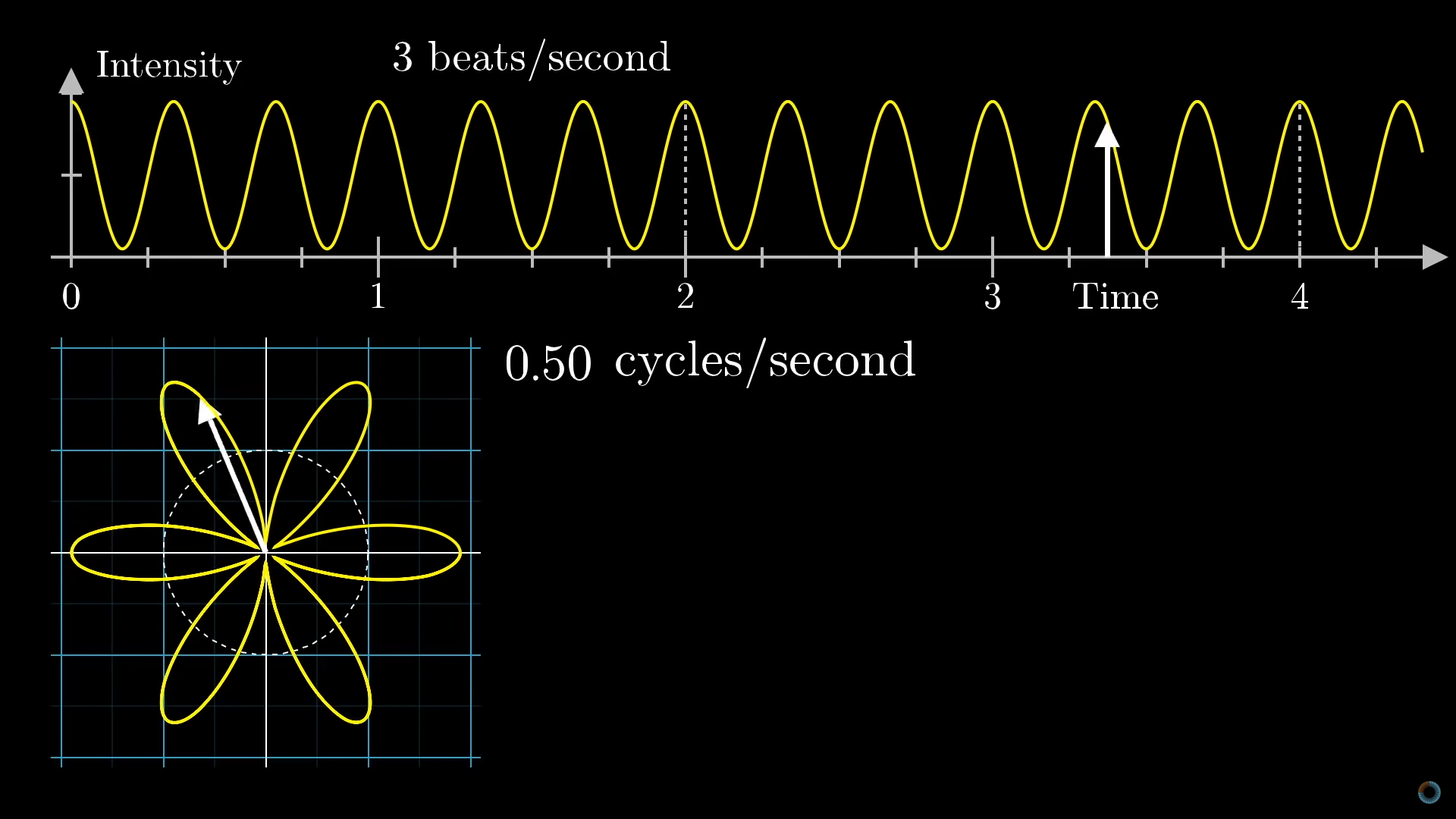
結論から述べると、動画の 3 分くらいのところで述べられているように、横軸が時間で縦軸が振幅となっているように波がある時、時間軸を角度、振幅を中心からの距離とみなして以下の図のように原点に巻き付けてみる。この時、一周分巻くのに何秒分使うか(cycles/second)によって見える図形が変化する。これによって得られる図形の重心を cycles/second 毎に調べていくと、元の波にどんな周波数の波が含まれているか分かるようだ。
簡単な例
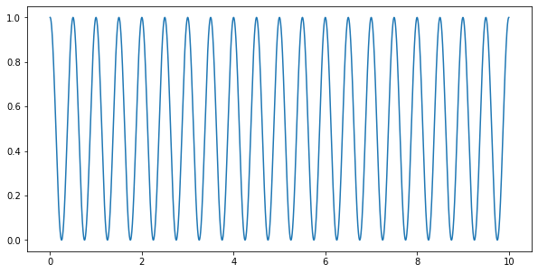
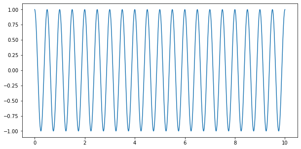
まずは簡単な例として cos(2πx) の波を作って実験してみる。動画のように 0 以上となるようにシフトしておく。(ついでに必要なのをimport)
import numpy as np
import matplotlib.pyplot as plt
from matplotlib.animation import FuncAnimation

# 時間 t を生成
n = 10000
t = np.linspace(0, 10, n)
# g(t) は cos(hz*2πt) を上にシフトした波
hz = 2
g = lambda t: (np.cos(hz * 2 * np.pi * t) + 1) / 2
gt = g(t)
# 描画
plt.figure(figsize=(10, 5))
plt.plot(t, gt)
plt.show()
生成した波はこちら。ちゃんとできてますね。
そして原点に cycles/second を変化させながら巻き付け重心を求める処理は、みんな大好き三角関数を用いて作成すると以下の visualized_fourier_transform 関数のように書ける。まぁこの処理は、各時刻の角度 theta を計算し、それに sin 関数と cos 関数、振幅である gt を用いて 2 次元平面上の x, y に写像しているだけなので比較的わかりやすい。
実際に動かしてみると gif が生成されるので載せておく。この時重心が大きく中心からずれるタイミングが二回ほどあり、1回目が 0 以上とするためにシフトした影響で生じた 0 付近の時であり、2回目が波の周波数と cycles/second が一致した瞬間である。
def visualized_fourier_transform(i):
    """
    角周波数毎のフーリエ変換の可視化処理

    :param i: 参照する cycles_list のインデックス番号
    """

    # cycles/second を調整
    f = cycles_list[i]
    theta = 2 * np.pi * f * t
    # 巻き付けに相当する変換
    # ※ 簡単のため一旦は三角関数で変換
    a = np.cos(theta) * gt
    b = -np.sin(theta) * gt
    # 重心を求める
    real = np.mean(a)
    imag = np.mean(b)
    if len(out) < frames:
        out.append(real + imag*1j)
    # 描画
    plt.cla()
    plt.xlim(-1.2, 1.2)
    plt.ylim(-1.2, 1.2)
    plt.plot(a, b, color='b', zorder=1)
    plt.scatter(real, imag, color='r', s=10, zorder=2)


# 描画するフレーム数
frames = 200
# 0 ~ 5 cycles まで
cycles_list = np.linspace(0, 5, frames)
# フーリエ変換の結果をスタックするリスト
out = []
# アニメーションを作成
fig = plt.figure(figsize=(5, 5))
ani = FuncAnimation(fig, visualized_fourier_transform, frames=range(frames), interval=100)
ani.save("sample1.gif", writer="pillow")
out = np.array(out)
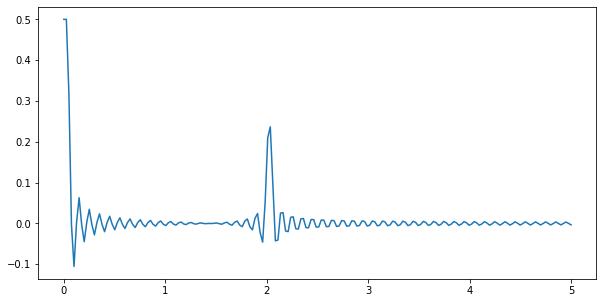
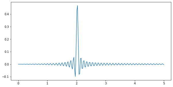
実際にどのタイミングで大きく重心が左右にずれるかを確認してみると確かに 0 と 2 のとこに大きな山があることが確認できます。現時点ではこのアイディアで「どんな周波数の波が含まれているかわかりそうだなぁ~」くらいにふむふむと眺めてもらえればと思います。
plt.figure(figsize=(10, 5))
plt.plot(cycles_list, out.real)
plt.show()
動画ではわかりにくくなるので 0 以上にすると言ってましたが、別にシフトしなくても同じ処理で変換して左右のずれを見ればよいのでやって結果を貼っておきます。
g = lambda t: np.cos(hz * 2 * np.pi * t)
gt = g(t)
plt.figure(figsize=(10, 5))
plt.plot(t, gt)
plt.show()
# フーリエ変換の結果をスタックするリスト
out = []
# アニメーションを作成
fig = plt.figure(figsize=(5, 5))
ani = FuncAnimation(fig, visualized_fourier_transform, frames=range(frames), interval=100)
ani.save("sample2.gif", writer="pillow")
out = np.array(out)
plt.figure(figsize=(10, 5))
plt.plot(cycles_list, out.real)
plt.show()
複雑な例
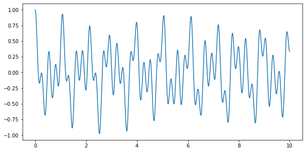
ちょっと複雑にして色んな周波数の波を混ぜてみます。今回は Hz = [1.5, 3, 4.75] の 3 つの波ですね。この時のポイントとして cycles/second の時の重心はそれぞれの波を個別に巻き付けた時の重心の和によって決まるという点です。先ほど確認したように、それぞれの波は周波数が一致したタイミングで山が発生し、それ以外は小さい値を持っていました。なので、このような波を作成しても各周波数に応じた山が出来上がるはずです。
Hz = [1.5, 3, 4.75]
g = lambda t: np.mean(np.array([np.cos(hz * 2 * np.pi * t) for hz in Hz]), axis=0)
gt = g(t)
plt.figure(figsize=(10, 5))
plt.plot(t, gt)
plt.show()
では早速アニメーションから。結構わちゃわちゃしてますねw
# フーリエ変換の結果をスタックするリスト
out = []
# アニメーションを作成
fig = plt.figure(figsize=(5, 5))
ani = FuncAnimation(fig, visualized_fourier_transform, frames=range(frames), interval=100)
ani.save("sample3.gif", writer="pillow")
out = np.array(out)
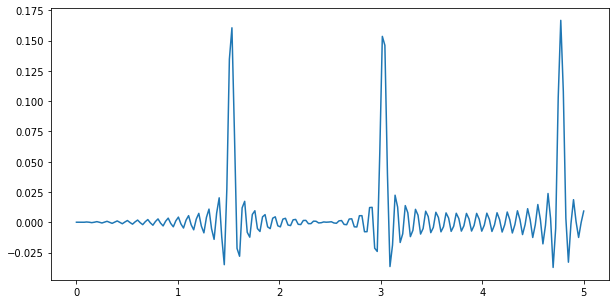
さて 3 回ほど横に大きくずれましたね!結果を見てみましょう。
plt.figure(figsize=(10, 5))
plt.plot(cycles_list, out.real)
plt.show()

なるほど…って感じです。
フーリエ変換との対応
ではここからはフーリエ変換とどのように対応しているかを確認していきましょう。wiki から式を取ってきつつ、参考にした動画と対応させながら調整すると以下の式になるかと思います。
$${\displaystyle {\hat {g}}(f):=\int _{-\infty }^{\infty }g(t)e^{-2\pi itf }dx}$$
説明の手順は動画と同様に複素平面上での円運動と確認した後、描画処理をフーリエ変換の形に置き換えていくことで説明していきます。
複素平面上での円運動
こちらに関しては以前記事にしたオイラーの公式の内容にもあるように以下が円運動なので、これがそのまま複素平面上での円運動であり、以下の式であれば x = 2 * np.pi * t * f と置くと f を調整することで円運動の速さを調整でき、それがそのまま巻き付ける回数を調整することに相当します。
$${\displaystyle e^{i x}=\cos x +i\sin x} $$
実際にその様子を確認できる処理を作成しておきました。f を 10 とすると 10 回転してくれます。ここを調整すれば回転の速度を変更できることが確認できるはずです。
def complex_plane(i):
    """
    複素平面での円運動

    :param i: 参照するインデックス番号
    """

    # f は周波数
    f = 10
    t = times[i]
    # 時計回りになるようマイナスをつける
    xy = np.e**(-2*np.pi*1j*f*t)
    # 描画
    plt.cla()
    plt.xlim(-1.2, 1.2)
    plt.ylim(-1.2, 1.2)
    plt.scatter(xy.real, xy.imag, color='r', s=10, zorder=2)


fig = plt.figure(figsize=(5, 5))
times = np.linspace(0, 1, frames)
ani = FuncAnimation(fig, complex_plane, frames=range(frames), interval=100)
ani.save("complex_plane.gif", writer="pillow")
可視化方法の変更
この円運動を使って巻き付けに相当する変換を書き換えてみます。するとほぼフーリエ変換の式
$${\displaystyle {\hat {g}}(f):=\int _{-\infty }^{\infty }g(t)e^{-2\pi itf }dx}$$
になったことが確認できるかと思います。積分の処理は重心を求める処理に相当しますが、今回は単に平均を取ったのでスケールは変化してしまっている点に注意が必要です。では最後に実際に可視化して先ほどの結果と一致することを確認して終わりにしましょう。
def visualized_fourier_transform(i):
    """
    角周波数毎のフーリエ変換の可視化処理

    :param i: 参照する cycles_list のインデックス番号
    """

    # cycles/second を調整
    f = cycles_list[i]
    # 巻き付けに相当する変換
    xy = gt * np.e**(-2*np.pi*1j*f*t)
    x = xy.real
    y = xy.imag
    # 重心を求める
    real = np.mean(x)
    imag = np.mean(y)
    if len(out) < frames:
        out.append(real + imag*1j)
    # 描画
    plt.cla()
    plt.xlim(-1.2, 1.2)
    plt.ylim(-1.2, 1.2)
    plt.plot(x, y, color='b', zorder=1)
    plt.scatter(real, imag, color='r', s=10, zorder=2)


# フーリエ変換の結果をスタックするリスト
out = []
# アニメーションを作成
fig = plt.figure(figsize=(5, 5))
ani = FuncAnimation(fig, visualized_fourier_transform, frames=range(frames), interval=100)
ani.save("sample5.gif", writer="pillow")
out = np.array(out)
plt.figure(figsize=(10, 5))
plt.plot(cycles_list, out.real)
plt.show()
なかなか概念として覚えやすくとてもいい動画でした。気になった方は動画の方も見てみてください。
まとめ
以前 Python: 離散フーリエ変換の実装 とか Python: 離散フーリエ変換(実装コードとテスト) とかを上げてましたが、まだまだ勉強不足だったようです。今回の実装は動画見ながら雑に作ったので粗が目立ちますが大きくは外れていないはずです。あくまで参考程度にどうぞ。最後に…こういうの実装するの楽しいよね(。-`ω-)
おまけ
最近流行りの ChatGPT にお願いしてコードを修正してもらった。
【私】
コメントを含めてわかりやすく修正できますか?それとも修正する必要はありませんか?
【ChatGPT】
このコードは比較的わかりやすいと思いますが、もう少しコメントを入れて説明を加えるとより分かりやすくなります。
下記のような修正を加えることができます:
def visualized_fourier_transform(i):
    """
    角周波数毎のフーリエ変換の可視化処理

    :param i: 参照する cycles_list のインデックス番号
    """
    # cycles/second を調整
    f = cycles_list[i]
    # 信号 g(t) の巻き付けに相当する変換を実施
    # xy は g(t) の変換結果の複素数表現
    xy = gt * np.e**(-2*np.pi*1j*f*t)
    # xy の Real 部分を x, Imag 部分を y として抽出
    x = xy.real
    y = xy.imag
    # x, y の平均値を求めて重心を求める
    real = np.mean(x)
    imag = np.mean(y)
    # 重心を out リストに格納
    if len(out) < frames:
        out.append(real + imag*1j)
    # 描画
    plt.cla()
    plt.xlim(-1.2, 1.2)
    plt.ylim(-1.2, 1.2)
    # x, y の値を折れ線グラフで描画
    plt.plot(x, y, color='b', zorder=1)
    # 重心を赤い点で描画
    plt.scatter(real, imag, color='r', s=10, zorder=2)
【私】
googleスタイルとNumPyスタイルの2種類のドックストリングを提示してください。
【ChatGPT】
Google スタイルのドックストリング:
def visualized_fourier_transform(i):
    """Visualize the Fourier transform for each angular frequency.

    Args:
        i (int): Index number of the reference cycles_list.

    """
    # Adjust cycles/second
    f = cycles_list[i]
    # Perform the equivalent transform for signal g(t)
    # xy represents the complex representation of the result of g(t)
    xy = gt * np.e**(-2*np.pi*1j*f*t)
    # Extract real part as x and imag part as y
    x = xy.real
    y = xy.imag
    # Calculate average to find the center of gravity
    real = np.mean(x)
    imag = np.mean(y)
    # Store center of gravity in out list
    if len(out) < frames:
        out.append(real + imag*1j)
    # Plotting
    plt.cla()
    plt.xlim(-1.2, 1.2)
    plt.ylim(-1.2, 1.2)
    # Plot x, y values as line graph
    plt.plot(x, y, color='b', zorder=1)
    # Plot center of gravity as red dot
    plt.scatter(real, imag, color='r', s=10, zorder=2)
NumPy スタイルのドックストリング:
def visualized_fourier_transform(i):
    """
    Visualize the Fourier transform for each angular frequency.

    Parameters
    ----------
    i : int
        Index number of the reference `cycles_list`.

    """
    # Adjust cycles/second
    f = cycles_list[i]
    # Perform the equivalent transform for signal g(t)
    # xy represents the complex representation of the result of g(t)
    xy = gt * np.exp(-2*np.pi*1j*f*t)
    # Extract real part as x and imag part as y
    x = xy.real
    y = xy.imag
    # Calculate average to find the center of gravity
    real = np.mean(x)
    imag = np.mean(y)
    # Store center of gravity in out list
    if len(out) < frames:
        out.append(real + imag*1j)
    # Plotting
    plt.cla()
    plt.xlim(-1.2, 1.2)
    plt.ylim(-1.2, 1.2)
    # Plot x, y values as line graph
    plt.plot(x, y, color='b', zorder=1)
    # Plot center of gravity as red dot
    plt.scatter(real, imag, color='r', s=10, zorder=2)
ほえー!英語になっちゃったけど便利ぃwちなみに記事の文章も修正してもらおうと思ったけど…それはあまり得意ではないみたい(´・ω・`)