MATLABで一瞬で線形判別機をつくる

Fisheriris を用いた判別分析のまとめ

MATLABのStatistics & Machine learning toolbox が最近便利になったときいて使ってみたメモ．あとで書き直す．
参考: https://jp.mathworks.com/help/stats/discriminant-analysis.html

データを読み込む

load fisheriris
%  meas         150x4              4800  double              
%  species      150x1             19300  cell    
%
%  meas については，1次元目が標本で，2次元目が特徴 (Sepal Length, Sepal Width, Petal Length, Petal Width)

判別機の学習と成績

usefeat = [1 2] % 使う特徴

% 使うデータを半々に分ける
idx = logical(ones(150,1));
meas_trn_idx = idx;
meas_trn_idx(1:2:150)=0;
meas_tst_idx=~meas_trn_idx;

nMdl = fitcdiscr(meas(meas_trn_idx,usefeat), species(meas_trn_idx));
[pres, score] = predict(nMdl, meas(meas_tst_idx,usefeat));

正解かどうか見てみる

disp([pres species(meas_tst_idx)]); % [予測されたクラス(pred) 正解クラス]
accuracy = sum(strcmp(pres, species(meas_tst_idx)))/length(pres);
disp(['正解率: ' num2str(accuracy)])
% 正解率は下記のような分類誤差を測るメソッド loss でも推定できる
L = nMdl.loss(meas(meas_tst_idx, usefeat), species(meas_tst_idx)); % 1-Lが正解率

最適化

• fitcdiscr は自動での grid search やベイズ最適化に対応している (2017aから？，デフォルトでは適用されない)
• これらを用いてより精度を上げることを試みることができる．
• ここではgammaについて最適なパラメータを探る

% Gamma (正則化パラメータ)
gm = 0.1:0.1:1;
for g = 1:length(gm)
    % 5-fold Cross Validation を行うオプションを追記
    % そのほかのオプションは doc fitcdiscr などで調べる
    oMdl{g} = fitcdiscr(meas(meas_trn_idx,usefeat), species(meas_trn_idx), ...
        'Gamma', gm(g), 'CrossVal','on', 'KFold', 5);   

    acc(g) = 1 - oMdl{g}.kfoldLoss;
end
[~,Mid] = max(acc);

最適化したパラメータでテストデータを弁別してみる

bMdl = fitcdiscr(meas(meas_trn_idx,usefeat), species(meas_trn_idx), 'gamma', gm(Mid));
Lo   = bMdl.loss(meas(meas_tst_idx, usefeat), species(meas_tst_idx));

% おそらく正解率が4%ほど上がっていると思う
disp(1-L)  % 最適化有り
disp(1-Lo) % 最適化なし

各特徴量での分布

bin1 = linspace(min(meas(:,1)), max(meas(:,1)), 25);
bin2 = linspace(min(meas(:,2)), max(meas(:,2)), 15);

% histogram
figure;
for sp = 1:3
    subplot(2,1,1); hold on;
    histogram(meas(strcmp(species, nMdl.ClassNames{sp}), 1), bin1)
    subplot(2,1,2); hold on;
    histogram(meas(strcmp(species, nMdl.ClassNames{sp}), 2), bin2)
end

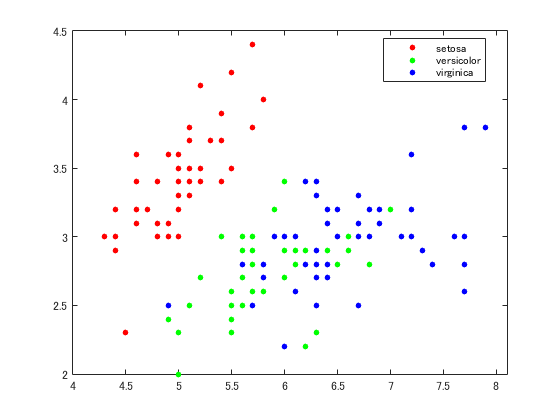
% scatter plot
figure; % scatterhist などでも可
gscatter(meas(:,1), meas(:,2), species)

% 事後確率を見てみる
[~, pprob] = bMdl.predict(meas(meas_tst_idx, usefeat));
imagesc(pprob); 

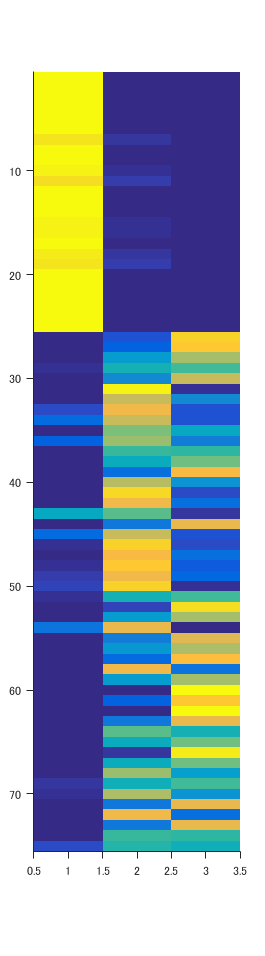
scatter での印象通り，事後確率をみてもこの二つの特徴量ではversicolor と virginica の判別が比較的難しいっぽいことが分かる