ふと、scikit-learn の使い方を人に説明したくなったので説明します。scikit-learn は機械学習で標準的に使われている Python のライブラリです。さまざまなモデルを統一した方法で操作できるので、数式が全く読めなくても使うだけなら他人が書いたコードも簡単に使えるという素晴らしい仕組みです。
まず本家ウェブサイト https://scikit-learn.org に行くと、Classification, Regression, Clustering という風にどんな事に使えるか紹介があります。ここでは Regression の一番上のサワリだけをやります。
糖尿病進行度予測の例
多分いきなり例を見た方が分かりやすいので例 Linear Regression Example に行きましょう。まずライブラリを読み込み、
from sklearn.datasets import load_diabetes
from sklearn.linear_model import LinearRegression
from sklearn.metrics import mean_squared_error, r2_score
import matplotlib.pyplot as plt
糖尿病データセット Diabetes dataset というのを読み込みます。
これは糖尿病患者の年齢や性別、コレステロール値などから、一年後どれくらい糖尿病が進行したかの記録です。
diabetes_X, result_y = load_diabetes(return_X_y=True, as_frame=True)
まず、入力となる患者データを確認します。これらの特徴量はすべて平均値で中心化され、標準偏差でスケーリングされています。なので例えば二人目の人の age が -0.001882 というのは -0.001882 歳ではなく、平均よりちょっと若い人という意味です。
- 年齢 (age):患者の年齢。
- 性別 (sex):患者の性別。
- 体格指数 (BMI - body mass index):患者の体重と身長を基に計算される体格指数。
- 平均血圧 (bp - average blood pressure):患者の平均血圧。
- S1:血清中の総コレステロール値(総コレステロールを表す可能性がある)。
- S2:低密度リポタンパク(LDL)値(「悪玉コレステロール」として知られる)。
- S3:高密度リポタンパク(HDL)値(「善玉コレステロール」として知られる)。
- S4:総コレステロールとHDLの比率。
- S5:血清トリグリセリドレベルの対数値。
- S6:血糖値。
diabetes_X
| age | sex | bmi | bp | s1 | s2 | s3 | s4 | s5 | s6 | |
|---|---|---|---|---|---|---|---|---|---|---|
| 0 | 0.038076 | 0.050680 | 0.061696 | 0.021872 | -0.044223 | -0.034821 | -0.043401 | -0.002592 | 0.019907 | -0.017646 |
| 1 | -0.001882 | -0.044642 | -0.051474 | -0.026328 | -0.008449 | -0.019163 | 0.074412 | -0.039493 | -0.068332 | -0.092204 |
| 2 | 0.085299 | 0.050680 | 0.044451 | -0.005670 | -0.045599 | -0.034194 | -0.032356 | -0.002592 | 0.002861 | -0.025930 |
| 3 | -0.089063 | -0.044642 | -0.011595 | -0.036656 | 0.012191 | 0.024991 | -0.036038 | 0.034309 | 0.022688 | -0.009362 |
| 4 | 0.005383 | -0.044642 | -0.036385 | 0.021872 | 0.003935 | 0.015596 | 0.008142 | -0.002592 | -0.031988 | -0.046641 |
| ... | ... | ... | ... | ... | ... | ... | ... | ... | ... | ... |
| 437 | 0.041708 | 0.050680 | 0.019662 | 0.059744 | -0.005697 | -0.002566 | -0.028674 | -0.002592 | 0.031193 | 0.007207 |
| 438 | -0.005515 | 0.050680 | -0.015906 | -0.067642 | 0.049341 | 0.079165 | -0.028674 | 0.034309 | -0.018114 | 0.044485 |
| 439 | 0.041708 | 0.050680 | -0.015906 | 0.017293 | -0.037344 | -0.013840 | -0.024993 | -0.011080 | -0.046883 | 0.015491 |
| 440 | -0.045472 | -0.044642 | 0.039062 | 0.001215 | 0.016318 | 0.015283 | -0.028674 | 0.026560 | 0.044529 | -0.025930 |
| 441 | -0.045472 | -0.044642 | -0.073030 | -0.081413 | 0.083740 | 0.027809 | 0.173816 | -0.039493 | -0.004222 | 0.003064 |
442 rows × 10 columns
この人たちが一年後どれくらい糖尿病が悪化したかを表す進行度も見てみます(この数値の求め方は書いてませんでした)。
result_y
0      151.0
1       75.0
2      141.0
3      206.0
4      135.0
       ...
437    178.0
438    104.0
439    132.0
440    220.0
441     57.0
Name: target, Length: 442, dtype: float64
BMI だけを使った予測
さてこのデータを利用して、BMI から糖尿病の一年後の悪化具合を予測するモデルを作ってみます。まず BMI だけ抜き出して、
bmi_X = diabetes_X[["bmi"]]
bmi_X
| bmi | |
|---|---|
| 0 | 0.061696 |
| 1 | -0.051474 |
| 2 | 0.044451 |
| 3 | -0.011595 |
| 4 | -0.036385 |
| ... | ... |
| 437 | 0.019662 |
| 438 | -0.015906 |
| 439 | -0.015906 |
| 440 | 0.039062 |
| 441 | -0.073030 |
442 rows × 1 columns
教師データ 422 件とテストデータ 20 件に分ます。テストデータは後でモデルの性能を測るのに使うので、学習に使うデータからより分けます。
# 入力を教師データとテストデータに分ける
bmi_X_train = bmi_X[:-20]
bmi_X_test = bmi_X[-20:]

# 出力を教師データとテストデータに分ける
result_y_train = result_y[:-20]
result_y_test = result_y[-20:]
いよいよモデルを作ります。
# Create linear regression object
model = LinearRegression()
model.fit(bmi_X_train, result_y_train)
より分けておいたテスト用データを使って予測します。
result_y_pred = model.predict(bmi_X_test)
print("Coefficients (係数または傾き w1):", model.coef_)
print("Intercept (切片 w0):", model.intercept_)
print()
print("つまり、モデルの式は 進行度 = %.2f + %.2f * BMI(正規化後) となる" % ((model.intercept_, model.coef_[0])))
print()
print("Mean squared error (平均二乗誤差): %.2f" % mean_squared_error(result_y_test, result_y_pred))
print("Root Mean squared error (平均二乗誤差平方根): %.2f" % (mean_squared_error(result_y_test, result_y_pred) / len(result_y_test)))
print("Coefficient of determination (決定係数 R2 (1 が完璧)): %.2f" % r2_score(result_y_test, result_y_pred))
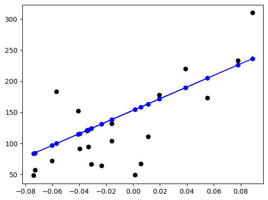
# Plot outputs
plt.scatter(bmi_X_test, result_y_test, color="black")
plt.plot(bmi_X_test, result_y_pred, color="blue", linewidth=1)
plt.scatter(bmi_X_test, result_y_pred, color="blue");
Coefficients (係数または傾き w1): [938.23786125]
Intercept (切片 w0): 152.91886182616113

つまり、モデルの式は 進行度 = 152.92 + 938.24 * BMI(正規化後) となる

Mean squared error (平均二乗誤差): 2548.07
Root Mean squared error (平均二乗誤差平方根): 127.40
Coefficient of determination (決定係数 R2 (1 が完璧)): 0.47
Scikit-Learn を使わないで線形回帰モデルを作る
この例では model.fit(教師データ入力, 教師データ出力) によって魔法のようにモデルが出来上がってしまいました。これでは面白く無いので、Scikit-Learn を使わなくてもモデルを作成できるか念の為確認してみます。 教科書によると、線形回帰モデル $y = a + b x$ は以下の式で求める事ができます。
$$
b = \frac{\sum_{i=1}^{n} (x_i - \bar{x})(y_i - \bar{y})}{\sum_{i=1}^{n} (x_i - \bar{x})^2}
$$
$$
a = \bar{y} - b \bar{x}
$$
変数の意味は以下です:
- $x$ BMI 教師データ
- $y$ 糖尿病進行度 教師データ
- $\bar{x}$ は $x$ の平均
- $\bar{y}$ は $y$ の平均
- $a$ y 切片
- $b$ 傾き
まず $x_i - \bar{x}$ です。
bmi_X_delta = bmi_X_train["bmi"] - bmi_X_train["bmi"].mean()
bmi_X_delta
0      0.061223
1     -0.051947
2      0.043978
3     -0.012068
4     -0.036858
         ...
417    0.070924
418   -0.025002
419   -0.055180
420   -0.036858
421    0.015955
Name: bmi, Length: 422, dtype: float64
次に $y_i - \bar{y}$ です。
result_y_delta = result_y_train - result_y_train.mean()
result_y_delta
0       -2.362559
1      -78.362559
2      -12.362559
3       52.637441
4      -18.362559
          ...
417    -98.362559
418    -69.362559
419   -111.362559
420     -7.362559
421     58.637441
Name: target, Length: 422, dtype: float64
さらに傾き
$$
b = \frac{\sum_{i=1}^{n} (x_i - \bar{x})(y_i - \bar{y})}{\sum_{i=1}^{n} (x_i - \bar{x})^2}
$$
を求めます。ここでズルして numpy の内積演算子 @ を使うと楽です。
b = (bmi_X_delta @ result_y_delta) / (bmi_X_delta @ bmi_X_delta)
b
938.2378612513513
最後に y 切片 $a = \bar{y} - b \bar{x}$ を求めます。
a = result_y_train.mean() - b * bmi_X_train["bmi"].mean()
a
152.91886182616113
この値を使って予測します。予測結果 result_pred_hand をプロットした青い線は Scikit-Learn を使った物と同じになりました。
result_pred_hand = a + bmi_X_test * b

# Plot outputs
plt.scatter(bmi_X_test, result_y_test, color="black")
plt.plot(bmi_X_test, result_pred_hand, color="blue", linewidth=1)
plt.scatter(bmi_X_test, result_pred_hand, color="blue");

線形モデルの定義
さて、元のドキュメントに戻って一番上の 1.1. Linear Models (線形モデル) の説明によると。線形モデルとは、↓のような式のことです。
$$
\hat{y}(w, x) = w_0 + w_1 x_1 + ... + w_p x_p
$$
変数の意味は次のようになります。
- $\hat{y}$: 出力予測値/従属変数 (一般的に実際の観測値を $y$ と表し予測値は $\hat{y}$ のように ^ を付けて区別します。)
- $x$: 入力値/説明変数
- $w$: 各特徴量に対応する重み
- BMI から糖尿病進行度を予測する例の場合 $w_0$ = 152.9, $w_1$ = 938.2
すべてのパラメータを使った予測
この例では分かりやすさのために BMI だけで糖尿病進行度を予測しましたが、複数の入力で予測モデルを作る事も出来ます。多少結果が良くなります。
# 入力を学習データとテストデータに分ける
diabetes_X_train = diabetes_X[:-20]
diabetes_X_test = diabetes_X[-20:]

# モデル作成
model_all = LinearRegression()
model_all.fit(diabetes_X_train, result_y_train)
result_y_pred = model_all.predict(diabetes_X_test)

print("Coefficients (係数または傾き):", model_all.coef_)
print("Intercept (切片 w0):", model_all.intercept_)
print()
print(f"つまり、モデルの式は 進行度 = {model_all.intercept_:.2f} +",
      "+".join([f" {coef:.2f} * X{index} " for index, coef in enumerate(model_all.coef_)]),
      "となる")
print()
print("Mean squared error (平均二乗誤差): %.2f" % mean_squared_error(result_y_test, result_y_pred))
print("Root Mean squared error (平均二乗誤差平方根): %.2f" % (mean_squared_error(result_y_test, result_y_pred) / len(result_y_test)))

print("Coefficient of determination (決定係数 R2 (1 が完璧)): %.2f" % r2_score(result_y_test, result_y_pred))
Coefficients (係数または傾き): [ 3.06094248e-01 -2.37635570e+02  5.10538048e+02  3.27729878e+02
 -8.14111926e+02  4.92799595e+02  1.02841240e+02  1.84603496e+02
  7.43509388e+02  7.60966464e+01]
Intercept (切片 w0): 152.76429169049118

つまり、モデルの式は 進行度 = 152.76 +  0.31 * X0 + -237.64 * X1 + 510.54 * X2 + 327.73 * X3 + -814.11 * X4 + 492.80 * X5 + 102.84 * X6 + 184.60 * X7 + 743.51 * X8 + 76.10 * X9  となる

Mean squared error (平均二乗誤差): 2004.52
Root Mean squared error (平均二乗誤差平方根): 100.23
Coefficient of determination (決定係数 R2 (1 が完璧)): 0.59