理解を深めるために勉強した結果を備忘録として残しておきます。

追記：TensorFlow Probability を使わない場合の内容の記事を書きました。
https://qiita.com/pocokhc/items/4fb37b39eaaed5a66d6d

問題設定

今回実験するために問題モデルは２つ用意しました。
１つは確率モデルを扱うためのシンプルなガウス分布、２つ目は異なる２つの確率分布が混じった分布になります。

これらのモデルを機械学習(Tensorflow)で学習していきます。

import

import numpy as np
import matplotlib.pyplot as plt
import seaborn as sns

問題１、ガウス分布による乱数モデル

問題１は、xの値で線形に平均と分散（ばらつき）が上がっていくガウス分布の乱数モデルです。
（分散といっていますが引数の scale は標準偏差の指定になります）

def target_model1(x):
    return np.random.normal(loc=x, scale=x)

描画すると以下です。

x_true1 = []
y_true1 = []
for x in np.linspace(0.1, 1.0, 200):
    x_true1.append(x)
    y_true1.append(target_model1(x))
x_true1 = np.asarray(x_true1)  # 今後のためにnumpy化

# 実際の値と平均の描画
plt.scatter(x_true1, y_true1, s=10, label="y")
plt.plot(x_true1, x_true1, label="mean")
plt.legend()
plt.show()

# 標準偏差の描画
plt.plot(x_true1, x_true1)
plt.title("standard deviation")
plt.show()

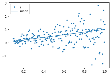
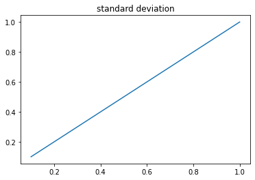
平均だけではなく分散（ばらつき）も大きくなっていくのでどんどんバラバラになっていく様子が見れるかと思います。

問題２、2種類のガウス分布による乱数モデル

問題２は、２つの確率モデルを混ぜた形です。
正方向は分散は固定にし、まっすぐに近い形になります。
負方向はばらつきがだんだん大きくなるモデルです。

def target_model2(x):
    if np.random.random() < 0.5:
        return np.random.normal(loc=x, scale=0.01)
    else:
        return np.random.normal(loc=-x, scale=x)

描画すると以下です。

x_true2 = []
y_true2 = []
for x in np.linspace(0.1, 1.0, 200):
    x_true2.append(x)
    y_true2.append(target_model2(x))
x_true2 = np.asarray(x_true2)  # 今後のためにnumpy化

# 実際の値と平均の描画
plt.scatter(x_true2, y_true2, s=10, label="y")
plt.plot(x_true2, x_true2, color="C1", label="positive mean")
plt.plot(x_true2, -x_true2, color="C2", label="negative mean")
plt.legend()
plt.show()

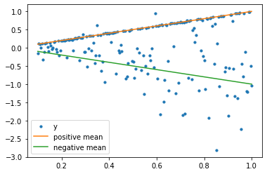
正方向はほとんど平均どおりのプロットになっていますが、負方向の点はバラバラになっていますね。

1.回帰モデル

まずは確率を扱わない回帰から見ていき、ガウス過程と比較したいと思います。

データ生成

学習に使うデータはランダムに取得します。
このデータを元に教師あり学習としてモデルを学習させます。

# 問題1の学習データ
x_train1 = []
y_train1 = []
for x in np.random.uniform(0.1, 1.0, 10000):
    x_train1.append(x)
    y_train1.append(target_model1(x))
x_train1 = np.asarray(x_train1)
y_train1 = np.asarray(y_train1)

# 問題2の学習データ
x_train2 = []
y_train2 = []
for x in np.random.uniform(0.1, 1.0, 10000):
    x_train2.append(x)
    y_train2.append(target_model2(x))
x_train2 = np.asarray(x_train2)
y_train2 = np.asarray(y_train2)

（決定的な）モデルの学習

教師あり学習だと一番使われるやり方ですね。
loss は回帰分析を想定しているので平均二乗誤差(mse)を指定します。
なので学習結果としては平均が学習されるはずです。

import tensorflow.keras as keras
from tensorflow.keras import layers as kl

model1 = keras.Sequential(
    [
        kl.Input(shape=(1,)),
        kl.Dense(64, activation="relu"),
        kl.Dense(64, activation="relu"),
        kl.Dense(1),
    ]
)
model1.compile(optimizer="adam", loss="mse")

以下で学習します。

model1.fit(x_train1, y_train1, epochs=5, batch_size=32)

学習結果

学習済みモデルから予測してみます。

# 予測
pred_y = model1(x_true1.reshape(-1, 1)).numpy().reshape(-1)

# 描画
plt.plot(x_true1, x_true1, label="mean")
plt.scatter(x_true1, y_true1, s=5, alpha=0.3, label="true y")
plt.scatter(x_true1, pred_y, s=5, label="pred y")
plt.legend()
plt.show()

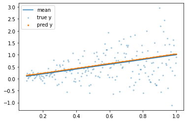
綺麗に平均上にプロットされていますね。

2.ガウス過程

1では平均しか学習できず、分散（散らばりぐらい）を学習できませんでした。
ガウス過程では確率的なモデル（ガウス分布）を仮定する事でこれを解決します。

理論に関しては説明するほど詳しくないので実装の話をメインで書きます。

ガウス過程モデル(TensorFlow Probability)

Tensorflow には確率的なモデルを扱うTensorFlow Probabilityがあるのでそちらを使います。

pip install tensorflow-probability

使い方ですが、Layerの最後の層に Dense+MixtureNormal層を追加するようです。
Dense層のユニット数は MixtureNormal.params_size で計算します。

import tensorflow_probability as tfp
tfpl = tfp.layers

num_components = 1  # 仮定するガウス分布の数
event_shape = (1,)  # 出力shape

# denseのユニット数を計算
params_size = tfpl.MixtureNormal.params_size(num_components, event_shape)

model2 = keras.Sequential(
    [
        kl.Input(shape=(1,)),
        kl.Dense(64, activation="relu"),
        kl.Dense(64, activation="relu"),
        kl.Dense(params_size, activation=None),  # 指定のDense層を追加(activationはNone)
        tfpl.MixtureNormal(num_components, event_shape)  # MixtureNormal層を最後に追加
    ]
)

また確率的な予測ではlossが変わります。
目的が誤差の最小化ではなく、確率尤度の最大化となります。

確率尤度の最大化は対数を取っても問題ないため、計算を簡単にするため一般的には対数化をします。

# 対数尤度を最大化するように学習
negative_log_likelihood = lambda y, q: -q.log_prob(y)
model2.compile(optimizer="adam", loss=negative_log_likelihood)

# 学習
model2.fit(x_train, y_train, epochs=5, batch_size=32)

学習結果

学習したガウス分布の平均と標準偏差の値も確認できたので見てみました。

# 予測
y = model2(x_true1.reshape(-1, 1))
pred_mean = y.mean().numpy().reshape(-1)
pred_stddev = y.stddev().numpy().reshape(-1)
pred_y = y.sample().numpy().reshape(-1)

# 描画
plt.plot(x_true1, x_true1, label="mean")
plt.scatter(x_true1, y_true1, s=5, alpha=0.3, label="true y")
plt.scatter(x_true1, pred_y, s=5, label="pred y")
plt.legend()
plt.show()

# 平均
plt.plot(x_true1, x_true1, label="true mean")
plt.plot(x_true1, pred_mean, label="pred mean")
plt.legend()
plt.show()

# 標準偏差
plt.plot(x_true1, x_true1, label="true stddev")
plt.plot(x_true1, pred_stddev, label="pred stddev")
plt.legend()
plt.show()

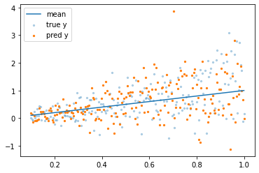
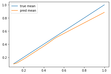
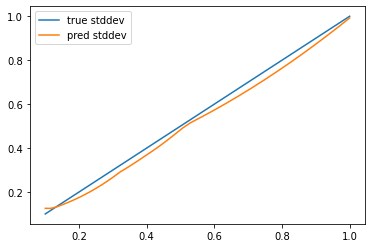
分散も含めてちゃんと学習できていますね。

問題２の学習結果

問題２側も同様に学習してみます。

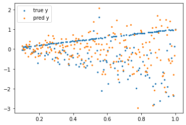
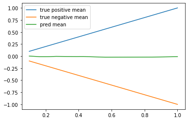
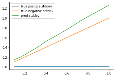
見てわかる通り、2つの確率モデルが含まれると学習できなくなります。
（正方向の予測値が全くできていません）

コード

num_components = 1
event_shape = (1,)
params_size = tfpl.MixtureNormal.params_size(num_components, event_shape)
model2_2 = keras.Sequential(
    [
        kl.Input(shape=(1,)),
        kl.Dense(64, activation="relu"),
        kl.Dense(64, activation="relu"),
        kl.Dense(params_size, activation=None),
        tfpl.MixtureNormal(num_components, event_shape)
    ]
)
negative_log_likelihood = lambda y, q: -q.log_prob(y)
model2_2.compile(optimizer="adam", loss=negative_log_likelihood)

# 問題２で学習
model2_2.fit(x_train2, y_train2, epochs=5, batch_size=32)

y = model2_2(x_true2.reshape(-1, 1))
pred_mean = y.mean().numpy().reshape(-1)
pred_stddev = y.stddev().numpy().reshape(-1)
pred_y = y.sample().numpy().reshape(-1)

# 描画
plt.scatter(x_true2, y_true2, s=5, label="true y")
plt.scatter(x_true2, pred_y, s=5, label="pred y")
plt.legend()
plt.show()

# 平均
plt.plot(x_true2, x_true2, label="true positive mean")
plt.plot(x_true2, -x_true2, label="true negative mean")
plt.plot(x_true2, pred_mean, label="pred mean")
plt.legend()
plt.show()

# 標準偏差
plt.plot(x_true2, [0.01 for _ in range(len(x_true2))], label="true positive stddev")
plt.plot(x_true2, x_true2, label="true negative stddev")
plt.plot(x_true2, pred_stddev, label="pred stddev")
plt.legend()
plt.show()

3.混合ガウス過程

混合ガウスモデル (GMM: Gaussian mixture model)は複数のガウス分布から予測するモデルです。
イメージは以下で、ガウス分布が1つだと1つの山しか学習できませんが、複数あれば山がたくさんあっても学習できるイメージです。
(ここでいう山は各確率分布の数の事を指します)

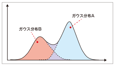
引用：https://xtrend.nikkei.com/atcl/contents/18/00076/00009/

コードとしては num_components がガウス分布の数になるのでここを変えるだけです。

num_components = 2  # 2に変える
event_shape = (1,)

params_size = tfpl.MixtureNormal.params_size(num_components, event_shape)
model3 = keras.Sequential(
    [
        kl.Input(shape=(1,)),
        kl.Dense(64, activation="relu"),
        kl.Dense(64, activation="relu"),
        kl.Dense(params_size, activation=None),
        tfpl.MixtureNormal(num_components, event_shape)
    ]
)
negative_log_likelihood = lambda y, q: -q.log_prob(y)
model3.compile(optimizer="adam", loss=negative_log_likelihood)

# 学習
model3.fit(x_train2, y_train2, epochs=5, batch_size=32)

# 学習後の予測
pred_y = model3(x_true2.reshape(-1, 1)).sample().numpy().reshape(-1)

# 予測結果の描画
plt.scatter(x_true2, y_true2, s=5, label="true y")
plt.scatter(x_true2, pred_y, s=5, label="pred y")
plt.legend()
plt.show()

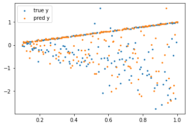
先ほどうまく学習できなかった正側の分布がうまく学習できていますね。
本当はそれぞれの平均と分散も出してみたかったのですが、出す方法は見つけられませんでした。

おわりに

中の理論については明るくないのですが、あっさり実装できた印象です。
誰かの参考になれば幸いです。

参考

・Understanding Regression Loss Functions And Introduction to TensorFlow Probability
・tfp.layers.MixtureNormal

Tensorflowで作る簡単な混合ガウス過程

問題設定

問題１、ガウス分布による乱数モデル

問題２、2種類のガウス分布による乱数モデル

1.回帰モデル

データ生成

（決定的な）モデルの学習

学習結果

2.ガウス過程

ガウス過程モデル(TensorFlow Probability)

学習結果

問題２の学習結果

3.混合ガウス過程

おわりに

参考