参考URL:https://www.tensorflow.org/tutorials/keras/classification?hl=ja
目標
以下のことを行う
- 画像を分類するニューラルネットワークを構築する
- ニューラルネットワークを訓練する
- モデルの性能を評価する
準備
パッケージの用意
# TensorFlow と tf.keras のインポート
import tensorflow as tf
from tensorflow import keras

# ヘルパーライブラリのインポート
import numpy as np
import matplotlib.pyplot as plt
# tensorflowのver確認
print(tf.__version__)
2.3.0
データセットを用意
今回はFashion-MNISTを使用する
10カテゴリーの白黒画像70,000枚が含まれいる
それぞれは下図のような1枚に付き1種類の衣料品が写っている低解像度(28×28ピクセル)の画像
|
|
|
Figure 1. Fashion-MNIST samples (by Zalando, MIT License). |
画像は28×28のNumPy配列から構成されている
それぞれのピクセルの値は0から255の間の整数
ラベル(label)は、0から9までの整数の配列
それぞれの数字が下表のように、衣料品のクラス(class)に対応
| Label | Class |
|---|---|
| 0 | T-shirt/top |
| 1 | Trouser |
| 2 | Pullover |
| 3 | Dress |
| 4 | Coat |
| 5 | Sandal |
| 6 | Shirt |
| 7 | Sneaker |
| 8 | Bag |
| 9 | Ankle boot |
fashion_mnist = keras.datasets.fashion_mnist

(train_images, train_labels), (test_images, test_labels) = fashion_mnist.load_data()
画像はそれぞれ単一のラベルに分類される
データセットには上記のクラス名が含まれていないため、
後で画像を出力するときのためにクラス名を保存しておく
class_names = ['T-shirt/top', 'Trouser', 'Pullover', 'Dress', 'Coat',
               'Sandal', 'Shirt', 'Sneaker', 'Bag', 'Ankle boot']
データの観察
print(train_images.shape)
print(test_images.shape)
(60000, 28, 28)
(10000, 28, 28)
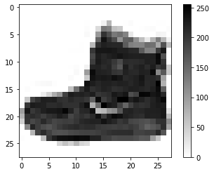
plt.figure()
plt.imshow(train_images[0], cmap=plt.cm.binary)
plt.colorbar()
plt.grid(False)
plt.show()
データの前処理
画像データの値を0から1までの範囲にスケール
train_images = train_images / 255.0

test_images = test_images / 255.0
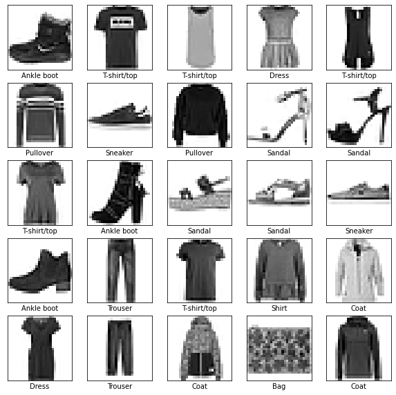
データの確認
plt.figure(figsize=(10,10))
for i in range(25):
    plt.subplot(5,5,i+1)
    plt.xticks([])
    plt.yticks([])
    plt.grid(False)
    plt.imshow(train_images[i], cmap=plt.cm.binary)
    plt.xlabel(class_names[train_labels[i]])
plt.show()
モデルの構築・学習
モデルの構築
- 28✖️28の2次元データを1次元に平滑(へいかつ)化
> tf.keras.layers.Flatten
> input_shape=(28, 28)で入力されるデータの形を指定している - 隠れ層の定義
> tf.keras.layers.Dense
> 128はユニットの数(ニューロンの数)
> activation='relu'は活性化関数ReLUを指定している
> 他の活性化関数:https://www.tensorflow.org/api_docs/python/tf/keras/activations?hl=ja - 全結合層の定義
> 最終的に10個クラスに分類するので10を指定する
> softmaxを活性化関数として使用しているので10個のノードは
> 今見ている画像が10個のクラスのひとつひとつに属する確率を出力する
model = keras.Sequential([
    keras.layers.Flatten(input_shape=(28, 28)),
    keras.layers.Dense(128, activation='relu'),
    keras.layers.Dense(10, activation='softmax')
])
モデルのコンパイル
学習のためのモデルを定義している
- optimizer:最適化アルゴリズム
- 今回は
Adamを指定 - その他の最適化アルゴリズム:https://www.tensorflow.org/api_docs/python/tf/keras/optimizers
- 今回は
- loss:損失関数
- 今回は
交差エントロピーを指定
- 今回は
- metrics:学習及びテスト中に定量化される項目
- 今回は
accuracy(正確性)を指定
- 今回は
model.compile(optimizer='adam',
              loss='sparse_categorical_crossentropy',
              metrics=['accuracy'])
モデルの訓練
model.fit(train_images, train_labels, epochs=5)
Epoch 1/5
1875/1875 [==============================] - 4s 2ms/step - loss: 0.4964 - accuracy: 0.8259
Epoch 2/5
1875/1875 [==============================] - 3s 2ms/step - loss: 0.3725 - accuracy: 0.8656
Epoch 3/5
1875/1875 [==============================] - 3s 2ms/step - loss: 0.3336 - accuracy: 0.8787
Epoch 4/5
1875/1875 [==============================] - 4s 2ms/step - loss: 0.3113 - accuracy: 0.8853
Epoch 5/5
1875/1875 [==============================] - 4s 2ms/step - loss: 0.2925 - accuracy: 0.8922


<tensorflow.python.keras.callbacks.History at 0x7f74fb8965f8>
評価
モデルを評価
テストデータを使用してモデルを評価する
test_loss, test_acc = model.evaluate(test_images,  test_labels, verbose=2)

print('\nTest accuracy:', test_acc)
313/313 - 0s - loss: 0.3479 - accuracy: 0.8780

Test accuracy: 0.878000020980835
予測
テストデータを学習したモデルで予測する
predictions = model.predict(test_images)
最初の画像の分類結果
確率として出力されている
predictions[0]
array([2.1071783e-06, 2.4513878e-07, 3.5516130e-09, 2.4936966e-07,
       6.1619041e-08, 6.4291209e-03, 3.7025956e-08, 2.2654539e-02,
       3.6237492e-07, 9.7091323e-01], dtype=float32)
# `np.argmax`で配列の中から最大の値(画像の分類されたラベルの番号)を取得
print(f'predicted label : {np.argmax(predictions[0])}')
# 正解データを確認
print(f'true label : {test_labels[0]}')
predicted label : 9
true label : 9
def plot_image(i, predictions_array, true_label, img):
    """
    画像を予測確率と共に表示
    """
    predictions_array, true_label, img = predictions_array[i], true_label[i], img[i]
    plt.grid(False)
    plt.xticks([])
    plt.yticks([])

    plt.imshow(img, cmap=plt.cm.binary)

    predicted_label = np.argmax(predictions_array)
    if predicted_label == true_label:
        color = 'blue'
    else:
        color = 'red'

    plt.xlabel("{} {:2.0f}% ({})".format(class_names[predicted_label],
                                    100*np.max(predictions_array),
                                    class_names[true_label]),
                                    color=color)

def plot_value_array(i, predictions_array, true_label):
    """
    予測結果の棒グラフを作成
    """
    predictions_array, true_label = predictions_array[i], true_label[i]
    plt.grid(False)
    plt.xticks([])
    plt.yticks([])
    thisplot = plt.bar(range(10), predictions_array, color="#777777")
    plt.ylim([0, 1])
    predicted_label = np.argmax(predictions_array)

    thisplot[predicted_label].set_color('red')
    thisplot[true_label].set_color('blue')
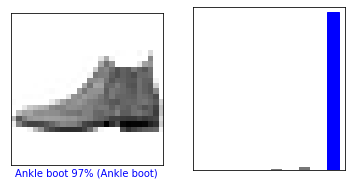
# テストデータの最初の画像で表示
i = 0
plt.figure(figsize=(6,3))
plt.subplot(1,2,1)
plot_image(i, predictions, test_labels, test_images)
plt.subplot(1,2,2)
plot_value_array(i, predictions,  test_labels)
plt.show()
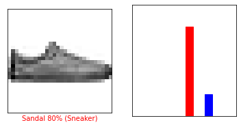
# テストデータの13番目の画像で表示
i = 12
plt.figure(figsize=(6,3))
plt.subplot(1,2,1)
plot_image(i, predictions, test_labels, test_images)
plt.subplot(1,2,2)
plot_value_array(i, predictions,  test_labels)
plt.show()
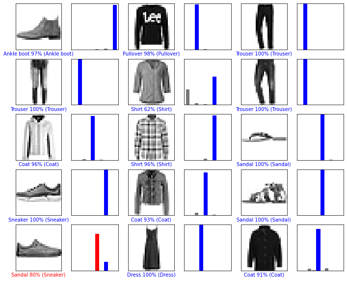
テストデータの15枚で描画を行う
num_rows = 5
num_cols = 3
num_images = num_rows*num_cols
plt.figure(figsize=(2*2*num_cols, 2*num_rows))
for i in range(num_images):
  plt.subplot(num_rows, 2*num_cols, 2*i+1)
  plot_image(i, predictions, test_labels, test_images)
  plt.subplot(num_rows, 2*num_cols, 2*i+2)
  plot_value_array(i, predictions, test_labels)
plt.show()
テストデータから画像を1枚取り出して予測を行う
img = test_images[0]

print(img.shape)
(28, 28)
tf.keras モデルは、サンプルの中のバッチ(batch)あるいは「集まり」について予測を行うように作られている。
そのため、1枚の画像を使う場合でも、リスト化する必要がある。
# 画像を1枚だけのバッチのメンバーにする
img = (np.expand_dims(img,0))

print(img.shape)
(1, 28, 28)
predictions_single = model.predict(img)

print(predictions_single)
[[2.1071742e-06 2.4513832e-07 3.5515995e-09 2.4936892e-07 6.1618806e-08
  6.4291116e-03 3.7025885e-08 2.2654528e-02 3.6237492e-07 9.7091323e-01]]
plot_value_array(0, predictions_single, test_labels)
_ = plt.xticks(range(10), class_names, rotation=45)
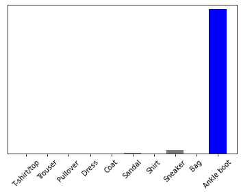
np.argmax(predictions_single[0])
9