はじめに
教師なし学習は一般的に教師あり学習と比較すると精度が落ちますが、その代わりに様々なメリットがあります。具体的に教師なし学習が役に立つシーンとして
**- パターンがあまりわかっていないデータ
- 時間的に変動するデータ
- 十分にラベルがついていないデータ**
などが挙げられます。
教師なし学習ではデータそのものから、データの背後にある構造を学習します。これによってラベルのついていないデータをより多く活用できるので、新たなアプリケーションへの道が開けるかもしれません。
前回、PCAとt-SNEを用いて教師なし学習で分類しました。
https://qiita.com/nakanakana12/items/af08b9f605a48cad3e4e
でもやっぱ流行りのディープラーニング使いたいですよね、ってことで今回の記事では
オートエンコーダを使った教師なし学習
を行います。
オートエンコーダ自体の詳しい説明は省略します。参考文献をご参照ください。
ライブラリのインポート
import keras
import random
import matplotlib.pyplot as plt
from matplotlib import cm
import seaborn as sns
import pandas as pd
import numpy as np
import plotly.express as px
import os

from sklearn.decomposition import PCA
from sklearn.cluster import KMeans
from sklearn.metrics import confusion_matrix
from sklearn.manifold import TSNE


from keras import backend as K
from keras.models import Sequential, Model, clone_model
from keras.layers import Activation, Dense, Dropout, Conv2D,MaxPooling2D,UpSampling2D
from keras import callbacks

from keras.layers import BatchNormalization, Input, Lambda
from keras import regularizers
from keras.losses import mse, binary_crossentropy

sns.set("talk")
データの準備
mnistのデータをダウンロードして前処理を行います。
前処理では正規化とチャネル位置の調整をしています。
fashion_mnist = keras.datasets.mnist
(train_images, train_labels), (test_images, test_labels) = fashion_mnist.load_data()

# 正規化
train_images = (train_images - train_images.min()) / (train_images.max() - train_images.min())
test_images = (test_images - test_images.min()) / (test_images.max() - test_images.min())

print(train_images.shape,test_images.shape)

# チャネル位置の調整
image_height, image_width = 28,28
train_images = train_images.reshape(train_images.shape[0],28*28)
test_images = test_images.reshape(test_images.shape[0],28*28)
print(train_images.shape, test_images.shape)
オートエンコーダの作成
オートエンコーダのモデルを作成します。
コード数がめちゃくちゃ少なくて感動しました。
ここでは36次元に圧縮するオートエンコーダを作成します。
全結合層を2つ繋げているのみで、一層目で36次元に圧縮、二層目でもとの大きさに戻す、という操作をしています。
つまり一層目がエンコーダ、二層目がデコーダになっています。
ここは書き方なども普通の教師あり学習と同じですね。
model = Sequential()

# エンコーダ
model.add(Dense(36, activation="relu", input_shape=(28*28,)))
# デコーダ
model.add(Dense(28*28,activation="sigmoid"))

model.compile(optimizer="adam",loss="binary_crossentropy")
model.summary()
オートエンコーダの学習
次にオートエンコーダを学習させます。
ここでのポイントとして、正解データはラベルではなく、画像データを用いているところです。
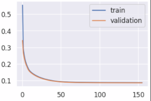
自分の環境では156epochで学習が完了しました。
fit_callbacks = [
    callbacks.EarlyStopping(monitor='val_loss',
                            patience=5,
                            mode='min')
]

# モデルを学習させる
# 正解データにtrain_imagesを用いる
model.fit(train_images, train_images,
          epochs=200,
          batch_size=2024,
          shuffle=True,
          validation_data=(test_images, test_images),
          callbacks=fit_callbacks,
          )
学習結果を確認してみます。損失が一定の値に収束しているのがわかりますね。
# テストデータの損失を確認
score = model.evaluate(test_images, test_images, verbose=0)
print('test xentropy:', score)

# テストデータの損失を可視化
score = model.evaluate(test_images, test_images, verbose=0)
print('test xentropy:', score)
オートエンコーダのモデル作成
次に先程のモデルからエンコーダ部分のみを取り出してモデルを作ります。
# 次元圧縮するモデル
encoder = clone_model(model)
encoder.compile(optimizer="adam", loss="binary_crossentropy")
encoder.set_weights(model.get_weights())
# 最後のレイヤーを削除
encoder.pop()
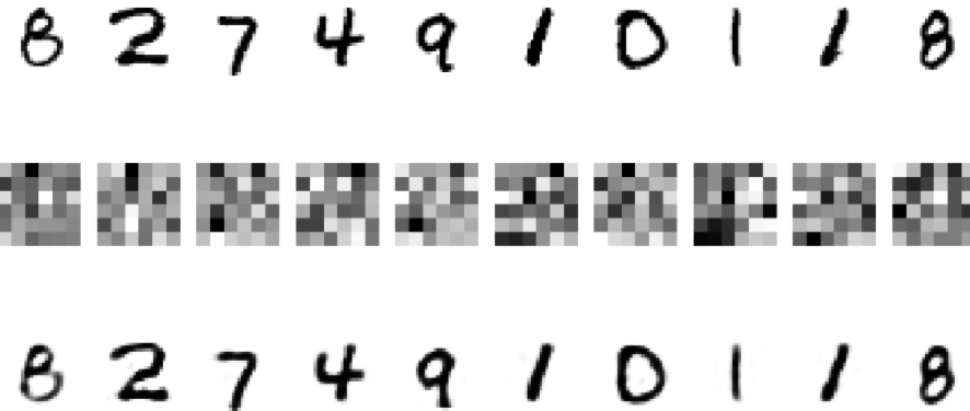
取り出したオートエンコーダを使って、36次元のデータを可視化します。
中間層では36次元の画像となっていますが、出力層では元のデータが復元されているのがわかります。
なんだか不思議ですね。
# テストデータから10点選んで可視化

p = np.random.randint(0, len(test_images), 10)
x_test_sampled = test_images[p]

# 選びだしたサンプルを AutoEncoder にかける
x_test_sampled_pred = model.predict(x_test_sampled,verbose=0)
# encoderのみにかける
x_test_sampled_enc = encoder.predict(x_test_sampled,verbose=0)

# 処理結果を可視化する
fig, ax = plt.subplots(3, 10,figsize=[20,10])
for i, label in enumerate(test_labels[p]):
    # 元画像
    img = x_test_sampled[i].reshape(image_height, image_width)
    ax[0][i].imshow(img, cmap=cm.gray_r)
    ax[0][i].axis('off')
    # AutoEncoder で次元圧縮した画像
    enc_img = x_test_sampled_enc[i].reshape(6, 6)
    ax[1][i].imshow(enc_img, cmap=cm.gray_r)
    ax[1][i].axis('off')
    # AutoEncoder で復元した画像
    pred_img = x_test_sampled_pred[i].reshape(image_height, image_width)
    ax[2][i].imshow(pred_img, cmap=cm.gray_r)
    ax[2][i].axis('off')
k-meansによる画像の分類
最後に36次元のデータを使ってk-meansによる分類を行います。
10個のクラスタに分類して、クラスタごとに最も多い数字を予測ラベルとしています。
# 次元削減したデータの作成
x_test_enc = encoder.predict(train_images)
print(x_test_enc.shape)

# k-menasによる分類
KM = KMeans(n_clusters = 10)
result = KM.fit(x_test_enc)

# 混同行列による評価
df_eval = pd.DataFrame(confusion_matrix(train_labels,result.labels_))
df_eval.columns = df_eval.idxmax()
df_eval = df_eval.sort_index(axis=1)
df_eval
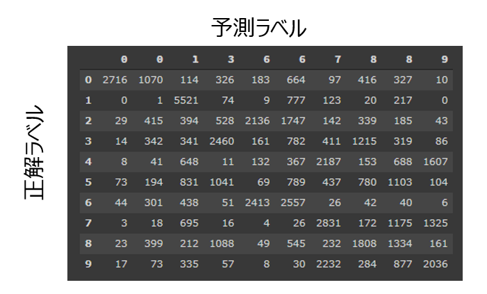
混同行列を確認すると、上手に10個には分類できなかったようです。
ここで、各クラスターの画像を可視化してみます。
# クラスターから5つずつ画像を表示する

fig, ax = plt.subplots(5,10,figsize=[15,8])
for col_i in range(10):
  idx_list = random.sample(set(np.where(result.labels_ == col_i)[0]), 5)
  ax[0][col_i].set_title("cluster:" + str(col_i), fontsize=12)
  for row_i, idx_i in enumerate(idx_list):
      ax[row_i][col_i].imshow((train_images[idx_i].reshape(image_height, image_width)), cmap=cm.gray_r)
      ax[row_i][col_i].axis('off')
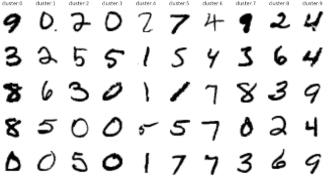
各クラスターをみると、数字が異なっていても画像的に似たような特徴があることがわかります。
例えばcluster 0は太くて、cluster 4は細いなどの特徴がありますね。
このことからラベルだけで表されるデータではなく、画像そのものから上手に特徴をとってこれていることがわかります。
ラベル外の情報で分類できるっていうのは面白いですね。新たなラベル付けなどができるということですもんね。
終わりに
今回はオートエンコーダを用いてmnistの数字を教師なし分類しました。
ラベルのデータ通りの分類はできなかったですが、クラスタを可視化するとラベル外の情報が浮き彫りになってきました。
ラベル外の情報を手に入れることができるというのが教師なし学習のすごいところですね。
参考になりましたらLGTMなどしていただけると励みになります。
参考文献
オートエンコーダとは?事前学習の仕組み・現在の活用方法を解説!!
https://it-trend.jp/development_tools/article/32-0024
KerasでAutoEncoder
https://qiita.com/fukuit/items/2f8bdbd36979fff96b07
Python: Keras で AutoEncoder を書いてみる
https://blog.amedama.jp/entry/keras-auto-encoder