kerasのFunctional APIを使ってseq2seqモデルを構築する モデル構築＆学習編

どんな記事？

深層学習のモデリングであれやこれや試してみたいけど、どうやって実装したらいいかわからん人向けに
割と自由度が高く、程よく抽象化されている枠組みとしてのkerasのfunctional APIを使って
sequentialでは難しいseq2seqをなるべくシンプルに実装してみる

目次

1. 概要編
2. 前処理編
3. モデル構築＆学習編（イマココ）
4. 推論編
5. モデル改良編　（まだ作ってない）

この記事のモチベーション

kerasを使えば深層学習の実装ができることはわかる。
具体的にはどういうコードを書けばいいのだろう？という疑問にお答えする。

モデル構築＆学習で必要なこと

kerasを使う場合、Modelクラスを活用すると便利です。
https://keras.io/ja/models/model/

Modelクラスは学習手法の定義、学習実行、学習により決まったモデルでの推論を担当します。

Modelインスタンスを作るためには、予め機械学習モデルが行う計算グラフを作っておく必要があります。
これにはsequential APIとfunctional APIの2つの選択肢があります。
sequential APIは非常にシンプルで、前のレイヤーの処理がそのまますべて次のレイヤーの処理になるような場合に有効です。
その代わりモデルの柔軟性を犠牲にしており、多入力多出力モデルなど複雑さが増してくると使えません。
functional APIはsequential APIに比べ、レイヤーどうしのつながりを自分で定義する必要がありますが、その分柔軟に記述できます。
今回はfunctional APIを用いたモデルを作ります。

計算グラフを構築してModelインスタンスを作ったらあとは簡単で
Modelインスタンスがもつcompileメソッドで学習方法の定義（最適化手法、損失関数の設定など）
fitメソッドで学習の実行ができます。

モデル構築＆学習の実装

計算グラフの定義

次の図で表すモデルを構築していきます

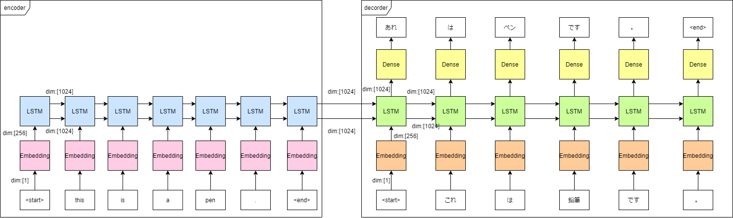
エンコーダー

エンコーダーでやるべきことは、入力のEmbedding、LSTMへの入力の2つ
実装例は以下

from keras.layers import Input, LSTM, Dense, Embedding
# Define an input sequence and process it.
encoder_inputs = Input(shape=(max_length_inp,),name='encoder_input')
encoder_inputs_embedding = Embedding(input_dim=vocab_inp_size, output_dim=embedding_dim)(encoder_inputs)
encoder = LSTM(units, return_state=True)
encoder_outputs, state_h, state_c = encoder(encoder_inputs_embedding)
# We discard `encoder_outputs` and only keep the states.
encoder_states = [state_h, state_c]

モデルへの入力はかならずInputレイヤーから行います。
ここで、Inputから入力文字列の最大長max_length_inp次元のデータを一度に入力してしまいます。
RNN系のアルゴリズムは入力のデータ列を1つずつ処理して順次次のステップに渡していきますが、このように略記することも可能です。

encoder_inputs_embedding = Embedding(input_dim=vocab_inp_size, output_dim=embedding_dim)(encoder_inputs)

の意味するところは
「input_dim=vocab_inp_size, output_dim=embedding_dimでEmbeddingレイヤーを定義する」
「定義されたEmbeddingにencoder_inputsを代入した結果がencoder_inputs_embeddingであるように計算グラフを追加する」
ということになります。

encoder = LSTM(units, return_state=True)
encoder_outputs, state_h, state_c = encoder(encoder_inputs_embedding)

のようにレイヤーの定義と計算グラフへの追加を別の行で行うこともできます。

デコーダー

デコーダーでやるべきことはデコーダー入力のEmbedding(teacher forcingのため)、LSTM、Denseの3つです。
実装例は以下

from keras.layers import Input, LSTM, Dense, Embedding
# Set up the decoder, using `encoder_states` as initial state.
decoder_inputs = Input(shape=(max_length_targ-1,),name='decoder_input')
decoder_inputs_embedding  = Embedding(input_dim=vocab_tar_size, output_dim=embedding_dim)(decoder_inputs)
# We set up our decoder to return full output sequences,
# and to return internal states as well. We don't use the
# return states in the training model, but we will use them in inference.
decoder_lstm = LSTM(units, return_sequences=True, return_state=True)
decoder_outputs, _, _ = decoder_lstm(decoder_inputs_embedding,
                                     initial_state=encoder_states)
decoder_dense = Dense(vocab_tar_size, activation='softmax')
decoder_outputs = decoder_dense(decoder_outputs)

エンコーダーと異なるところは
* Inputのshapeが1少ない。
* LSTMのreturn_sequences=Trueオプションを入れて、各ステップごとのLSTM出力を得ている
* LSTMがエンコーダーから得たLSTMの隠れ層の記憶encoder_statesを受け取っている
* Denseレイヤーがある。出力層なのでactivationはsoftmax

Modelインスタンスの生成

ここまでくればあとはstraight forwardです

from keras.models import Model
# Define the model that will turn
# `encoder_input_data` & `decoder_input_data` into `decoder_target_data`
model = Model([encoder_inputs, decoder_inputs], decoder_outputs)

生成されたモデルの確認

from IPython.display import SVG
SVG(model_to_dot(model).create(prog='dot', format='svg'))

でモデルを表す計算グラフを可視化できます。

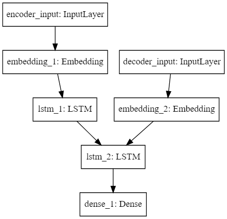
各レイヤーの描画上の位置関係は冒頭で見せた図とは違っていますが、ネットワークとしてみれば同じなことがわかります。

また、

model.summary()

で各レイヤーのパラメータ数などを確認できます。

__________________________________________________________________________________________________
Layer (type)                    Output Shape         Param #     Connected to                     
==================================================================================================
encoder_input (InputLayer)      (None, 18)           0                                            
__________________________________________________________________________________________________
decoder_input (InputLayer)      (None, 17)           0                                            
__________________________________________________________________________________________________
embedding_1 (Embedding)         (None, 18, 256)      1699328     encoder_input[0][0]              
__________________________________________________________________________________________________
embedding_2 (Embedding)         (None, 17, 256)      2247168     decoder_input[0][0]              
__________________________________________________________________________________________________
lstm_1 (LSTM)                   [(None, 1024), (None 5246976     embedding_1[0][0]                
__________________________________________________________________________________________________
lstm_2 (LSTM)                   [(None, 17, 1024), ( 5246976     embedding_2[0][0]                
                                                                 lstm_1[0][1]                     
                                                                 lstm_1[0][2]                     
__________________________________________________________________________________________________
dense_1 (Dense)                 (None, 17, 8778)     8997450     lstm_2[0][0]                     
==================================================================================================
Total params: 23,437,898
Trainable params: 23,437,898
Non-trainable params: 0
__________________________________________________________________________________________________

実際のモデリング時は適宜可視化していくとデバッグが捗るのでおすすめです。

学習条件の設定と学習実行

損失関数をクロスエントロピーとして、Adamを使って最適化したいと思います。
各エポックごとに単語の的中率を見ることにします。

5エポックごとにモデルを保存しようと思います。

実装例は以下

model.compile(optimizer='adam', loss='categorical_crossentropy',
              metrics=['accuracy'])

# define save condition
dir_path = 'saved_models/LSTM/'
save_every = 5
train_schedule = [save_every for i in range(divmod(epochs,save_every)[0])]
if divmod(epochs,save_every)[1] != 0:
    train_schedule += [divmod(epochs,save_every)[1]]

#run training
total_epochs = 0
for epoch in train_schedule:
    history = model.fit([encoder_input_tensor, decoder_input_tensor], 
                          np.apply_along_axis(lambda x: np_utils.to_categorical(x,num_classes=vocab_tar_size), 1, decoder_target_tensor),
                          batch_size=batch_size,
                          epochs=epoch,
                          validation_split=0.2)
    total_epochs += epoch
    filename = str(total_epochs) + 'epochs_LSTM.h5'
    model.save(dir_path+filename)

色々やってますが、キモはmodel.compileとmodel.fitだけです。ミニマムにはこの2つだけでいいかと思います。

model.compileにオプションとして最適化手法と損失関数と評価用のメトリックを渡します。
そうするとmodel.fitで学習実行します。
model.fitに与えるパラメータで特に重要なのは入力するデータと正解データです。
正解データがnp.apply_along_axis(lambda x: np_utils.to_categorical(x,num_classes=vocab_tar_size), 1, decoder_target_tensor)になっているのは
decoder_target_tensorの各要素をone-hot encodingした形式に変換したいがためです。

コーディング、デバッグ時のtips

適宜可視化をして次元の整合性を確認したり、適宜具体的な値を代入してみるとバグが早く見つかります。
それぞれのレイヤーは関数のように扱えるので具体的な値を代入すれば具体的な値の出力が得られます。

参考

前処理部分は下記
アテンションを用いたニューラル機械翻訳
https://www.tensorflow.org/tutorials/text/nmt_with_attention

学習・推論部分のコードのベースは下記
Sequence to sequence example in Keras (character-level).
https://keras.io/examples/lstm_seq2seq/

学習に使ったデータは下記
https://github.com/odashi/small_parallel_enja

本記事のコードが入ってるリポジトリ
https://github.com/nagiton/simple_NMT