基本の作図
例えばこんな感じのデータフレームがあったとする.
    x         y
0   2  0.954025
1   3  0.146810
2   1  0.409961
3   1  0.164558
4   3  0.782152
5   2  0.905869
6   3  0.210528
7   1  0.437970
8   1  0.801206
9   3  0.089576
10  2  0.960357
11  2  0.670732
このデータフレームから標準誤差付きの図を描こうとすると,こんな感じ.
import numpy as np
import matplotlib.pyplot as plt

m = df.pivot_table(index='x', values='y', aggfunc='mean')
e = df.pivot_table(index='x', values='y', aggfunc='sem')
m.plot(xlim=[0.8, 3.2], yerr=e)
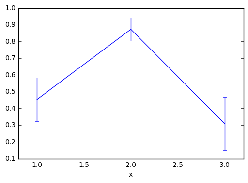
このように,yerrに誤差の大きさを指定することで,誤差棒を作成することができる.
信頼区間を用いた作図
そこで,信頼区間の長さを求めるcilenを定義して利用することにする.
import numpy as np
from scipy import stats
import matplotlib.pyplot as plt


def cilen(arr, alpha=0.95):
    if len(arr) <= 1:
        return 0
    m, e, df = np.mean(arr), stats.sem(arr), len(arr) - 1
    interval = stats.t.interval(alpha, df, loc=m, scale=e)
    cilen = np.max(interval) - np.mean(interval)
    return cilen

m = df.pivot_table(index='x', values='y', aggfunc='mean')
e = df.pivot_table(index='x', values='y', aggfunc=cilen)
m.plot(xlim=[0.8, 3.2], yerr=e)
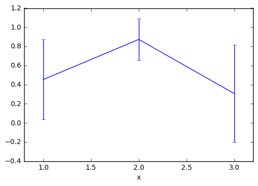
信頼区間付きの図を作成することができた.
おまけ
信頼区間を計算する方法は「nかn-1か」問題のせいでごちゃごちゃしてます.
「車輪の再発明は避けよ」に従って,とりあえず「信頼区間 Python」とかで検索した人は,
あたりを見て,微妙に違うことに困惑しつつも両方試してみて,そして結果が違うことに辟易することになると思います (なりました).
Rと同じ答えになるのは1の方.違うのは2の方です.ちょっと試してみます.
> x <- c(1, 1, 3, 3)
> t.test(x)

    One Sample t-test

data:  x
t = 3.4641, df = 3, p-value = 0.04052
alternative hypothesis: true mean is not equal to 0
95 percent confidence interval:
 0.1626138 3.8373862
sample estimates:
mean of x
        2
1の方法
import numpy as np
from scipy import stats

alpha     = 0.95
data = [1, 1, 3, 3]

mean_val = np.mean(data)
sem_val  = stats.sem(data)  # standared error of the mean
ci       = stats.t.interval(alpha, len(data)-1, loc=mean_val, scale=sem_val)

print(ci)

>> (0.16261376896260105, 3.837386231037399)
2の方法
import math
import numpy as np
from scipy import stats

alpha     = 0.95
data = [1, 1, 3, 3]

mean_val = np.mean(data)
std_val = np.std(data)
ci = stats.t.interval(alpha,len(data)-1,loc=mean_val,scale=std_val/math.sqrt(len(data)))
print(ci)

>> (0.40877684735786857, 3.5912231526421312)
今回は天下のRに従うことにしたので1を採用しています.
なお,2は何が違うのかというと,ciを計算する箇所の最後の方
math.sqrt(len(data))
これです.nで割ってます.しかし推測統計を行うのであればn-1で割った方が良いです.t分布を仮定するからですね.実際,
math.sqrt(len(data) - 1)
とすると,方法2の答えもRと完全に一致します.