始めに

chainerと似て抽象化がされている。
違いの一例としてはネットワークの定義でユニット数の書き方がchainerと逆になってる。Dense(1, input_dim=784,... 出力ユニット数,入力ユニット数の順になってる。
この記事では関数の紹介、使い方、どこで使われてるかを説明できる範囲で紹介します。
※layer_testというサンプルが多用されてますが、ただのテストコードなことに後で気づきましたので、そのうち直します。

継承関係

Layer
↑
Container
↑
Model
↑
Sequential

Keras v2では名前が変わったりしてます。
今はv1を元に書いています。
http://qiita.com/miyamotok0105/items/322b29339e1771184b9e

from keras.models import Sequential
from keras.layers import Dense, Activation

# for a single-input model with 2 classes (binary):                                                                                                           

model = Sequential()
model.add(Dense(1, input_dim=784, activation='sigmoid'))
model.compile(optimizer='rmsprop',
              loss='binary_crossentropy',
              metrics=['accuracy'])

# generate dummy data                                                                                                                                         
import numpy as np
data = np.random.random((1000, 784))
labels = np.random.randint(2, size=(1000, 1))

print(data.shape) #(1000, 784)
print(labels.shape) #(1000, 1)

# train the model, iterating on the data in batches                                                                                                           
# of 32 samples                                                                                                                                               
model.fit(data, labels, nb_epoch=10, batch_size=32)

実行すると学習される。

1000/1000 [==============================] - 1s - loss: 2.8725 - acc: 0.0950      
Epoch 2/10
1000/1000 [==============================] - 0s - loss: 2.5740 - acc: 0.1220     
Epoch 3/10
1000/1000 [==============================] - 0s - loss: 2.4748 - acc: 0.1430     
Epoch 4/10
1000/1000 [==============================] - 0s - loss: 2.3134 - acc: 0.1870     
Epoch 5/10
1000/1000 [==============================] - 0s - loss: 2.2782 - acc: 0.2010     
Epoch 6/10
1000/1000 [==============================] - 0s - loss: 2.1186 - acc: 0.2360     
Epoch 7/10
1000/1000 [==============================] - 0s - loss: 2.0329 - acc: 0.2920     
Epoch 8/10
1000/1000 [==============================] - 0s - loss: 1.9268 - acc: 0.3200     
Epoch 9/10
1000/1000 [==============================] - 0s - loss: 1.8635 - acc: 0.3170     
Epoch 10/10
1000/1000 [==============================] - 0s - loss: 1.7225 - acc: 0.4270

Sequential (系列) モデル

層を積み重ねたもの。

Merge層

簡単に層をマージできる。faster-rcnnやresnetなどマージしてる層で使えそう。

rom keras.models import Sequential
from keras.layers import Dense, Activation
from keras.layers import Merge, LSTM, Dense

# for a multi-input model with 10 classes:                                                                                                                    

left_branch = Sequential()
left_branch.add(Dense(32, input_dim=784))

right_branch = Sequential()
right_branch.add(Dense(32, input_dim=784))

merged = Merge([left_branch, right_branch], mode='concat')

model = Sequential()
model.add(merged)
model.add(Dense(10, activation='softmax'))

model.compile(optimizer='rmsprop',
              loss='categorical_crossentropy',
              metrics=['accuracy'])

# generate dummy data                                                                                                                                         
import numpy as np
from keras.utils.np_utils import to_categorical
data_1 = np.random.random((1000, 784))
data_2 = np.random.random((1000, 784))

# these are integers between 0 and 9                                                                                                                          
labels = np.random.randint(10, size=(1000, 1))
# we convert the labels to a binary matrix of size (1000, 10)                                                                                                 
# for use with categorical_crossentropy                                                                                                                       
labels = to_categorical(labels, 10)

# train the model                                                                                                                                             
# note that we are passing a list of Numpy arrays as training data                                                                                            
# since the model has 2 inputs                                                                                                                                
model.fit([data_1, data_2], labels, nb_epoch=10, batch_size=32)

多層パーセプトロン

from keras.models import Sequential
from keras.layers import Dense, Dropout, Activation
from keras.optimizers import SGD

model = Sequential()
# Dense(64) is a fully-connected layer with 64 hidden units.                                                                                                  
# in the first layer, you must specify the expected input data shape:                                                                                         
# here, 20-dimensional vectors.                                                                                                                               
model.add(Dense(64, input_dim=20, init='uniform'))
model.add(Activation('tanh'))
model.add(Dropout(0.5))
model.add(Dense(64, init='uniform'))
model.add(Activation('tanh'))
model.add(Dropout(0.5))
model.add(Dense(10, init='uniform'))
model.add(Activation('softmax'))

sgd = SGD(lr=0.1, decay=1e-6, momentum=0.9, nesterov=True)
model.compile(loss='categorical_crossentropy',
              optimizer=sgd,
              metrics=['accuracy'])

# generate dummy data                                                                                                                                         
import numpy as np
X_train = np.random.random((1000, 20))
y_train = np.random.randint(2, size=(1000, 10))

X_test = np.random.random((1000, 20))
y_test = np.random.randint(2, size=(1000, 10))


model.fit(X_train, y_train,
          nb_epoch=5,
          batch_size=16)
score = model.evaluate(X_test, y_test, batch_size=16)

次元が違うエラー

入力次元とネットワーク入力層の次元。出力次元とネットワーク出力層の次元。
がそれぞれ同じでないとエラーになる。

model.add(Dense(64, input_dim=20, init='uniform'))と20とX_train = np.random.random((1000, 20))の20は合わせる。出力も同様。

X_train = np.random.random((1000, 20))→X_train = np.random.random((1001, 20))
ValueError: Input arrays should have the same number of samples as target arrays. Found 1001 input samples and 1000 target samples.

y_train = np.random.randint(2, size=(1000, 10))→y_train = np.random.randint(2, size=(1000, 9))
ValueError: Error when checking model target: expected activation_3 to have shape (None, 10) but got array with shape (1000, 9)

LSTMを用いた系列データの分類

from keras.models import Sequential
from keras.layers import Dense, Dropout, Activation
from keras.layers import Embedding
from keras.layers import LSTM

model = Sequential()
model.add(Embedding(100, 256, input_length=256))
model.add(LSTM(output_dim=128, activation='sigmoid', inner_activation='hard_sigmoid'))
model.add(Dropout(0.5))
model.add(Dense(1))
model.add(Activation('sigmoid'))

model.compile(loss='binary_crossentropy',
              optimizer='rmsprop',
              metrics=['accuracy'])

# generate dummy data                                                                                                                                         
import numpy as np
X_train = np.random.random((10, 256))
Y_train = np.random.randint(2, size=(10, 1))

print(X_train.shape)
print(Y_train.shape)

model.fit(X_train, Y_train, batch_size=16, nb_epoch=1)

functional API

複数の出力があるモデルや有向非巡回グラフ、共有レイヤーを持ったモデルなどの複雑なモデルを定義するためのインターフェース。

モデルについて

シーケンシャルモデル，functional APIとともに用いるモデルクラス。

レイヤーについて

Coreレイヤー

Dense

通常の全結合ニューラルネットワークレイヤー

model = Sequential()
model.add(Dense(1, input_dim=784, activation='sigmoid'))

Activation

出力に活性化関数を適用

model = Sequential()
model.add(Dense(1, input_dim=784, activation='sigmoid'))

Dropout

過学習対応でランダムでユニットを重みを保存しない。

def create_model1():
    # create model
    model = Sequential()
    model.add(Dropout(0.2, input_shape=(60,)))
    model.add(Dense(60, init='normal', activation='relu', W_constraint=maxnorm(3)))
    model.add(Dense(30, init='normal', activation='relu', W_constraint=maxnorm(3)))
    model.add(Dense(1, init='normal', activation='sigmoid'))
    # Compile model
    sgd = SGD(lr=0.1, momentum=0.9, decay=0.0, nesterov=False)
    model.compile(loss='binary_crossentropy', optimizer=sgd, metrics=['accuracy'])
    return model

Flatten

入力を平坦化する．バッチサイズに影響されない。

    # we start off with an efficient embedding layer which maps
    # our vocab indices into embedding_dims dimensions
    model.add(Embedding(max_features,
                        embedding_dims,
                        input_length=maxlen,
                        dropout=0.2))

    # we add a Convolution1D, which will learn nb_filter
    # word group filters of size filter_length:
    model.add(Convolution1D(nb_filter=nb_filter,
                            filter_length=filter_length,
                            border_mode='valid',
                            activation='relu',
                            subsample_length=1))
    # we use max pooling:
    model.add(MaxPooling1D(pool_length=model.output_shape[1]))

    # We flatten the output of the conv layer,
    # so that we can add a vanilla dense layer:
    model.add(Flatten())

Reshape

ある型に出力を変形

    layer_test(core.Reshape,
               kwargs={'target_shape': (8, 1)},
               input_shape=(3, 2, 4))

Permute

与えられたパターンにより入力の次元を変更する．
例えば，RNNsやconvnetsの連結に対して役立ちます

    layer_test(core.Permute,
               kwargs={'dims': (2, 1)},
               input_shape=(3, 2, 4))

RepeatVector

n回入力を繰り返す．

    layer_test(core.RepeatVector,
               kwargs={'n': 3},
               input_shape=(3, 2))

Merge

model1 = Sequential()
model1.add(Dense(32))

model2 = Sequential()
model2.add(Dense(32))

merged_model = Sequential()
merged_model.add(Merge([model1, model2], mode='concat', concat_axis=1)

resnet

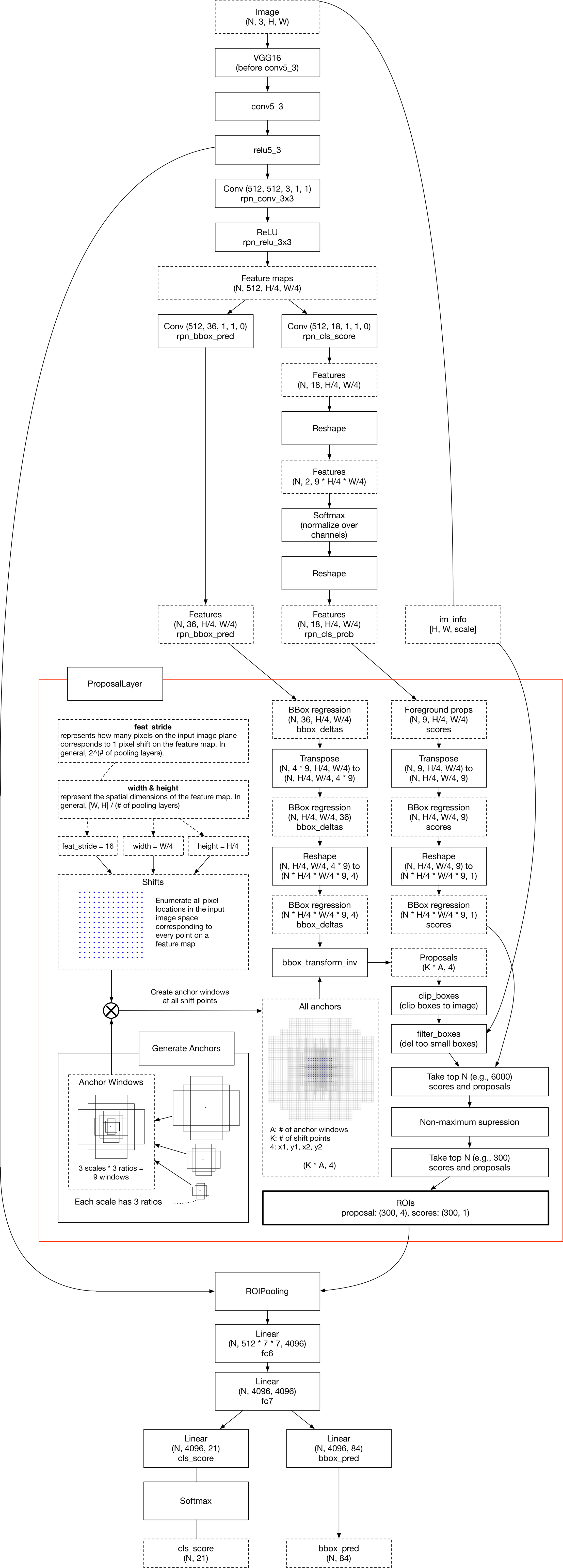
faster-rcnn

Lambda

簡易的にオリジナル層を追加できる。

# 一つのx -> x^2レイヤーを加える．
model.add(Lambda(lambda x: x ** 2))

例１
kerasバックエンドにあるtensorflowかtheanoの関数をほりこめる。
http://qiita.com/neka-nat@github/items/d0435d9c92cef2ee2901

from keras.models import Model
from keras.layers import Input, Lambda
import keras.backend as K

x_in = Input(shape=(3, 3))
x = Lambda(lambda x: K.abs(x))(x_in)
model = Model(input=x_in, output=x)

例２
https://keunwoochoi.wordpress.com/2016/11/18/for-beginners-writing-a-custom-keras-layer/

def output_of_lambda(input_shape):
    return (input_shape[0], 1, input_shape[2])

def mean(x):
    return K.mean(x, axis=1, keepdims=True)

model.add(Lambda(mean, output_shape=output_of_lambda))

例３
croppingレイヤーの追加

class Cropping2D(Layer):

      def call(self, x, mask=None):
    return x[:, :, self.cropping[0][0]:x._keras_shape[2]-self.cropping[0][1], self.cropping[1][0]:x._keras_shape[3]-self.cropping[1][1]]

      def get_config(self):
          config = {'cropping': self.padding}

ActivityRegularization

変化のない入力を通過するレイヤー，しかしアクティビティに基づいたコスト関数の更新を適用する．重み上限を付与。

    from keras.engine import Input, Model

    layer = core.ActivityRegularization(l1=0.01, l2=0.01)

    # test in functional API
    x = Input(shape=(3,))
    z = core.Dense(2)(x)
    y = layer(z)
    model = Model(input=x, output=y)
    model.compile('rmsprop', 'mse', mode='FAST_COMPILE')

    model.predict(np.random.random((2, 3)))

    # test serialization
    model_config = model.get_config()
    model = Model.from_config(model_config)
    model.compile('rmsprop', 'mse')

Masking

スキップされるタイムステップを特定するためのマスク値を使うことによって入力シーケンスをマスクする．
LSTMレイヤーに与えるための(samples, timesteps, features)の型のNumpy配列xを検討する．あなたが#3と#5のタイムステップに関してデータを欠損しているので，これらのタイムステップをマスクしたい場合，あなたは以下のようにできる:

set x[:, 3, :] = 0. and x[:, 5, :] = 0.
insert a Masking layer with mask_value=0. before the LSTM layer:

model = Sequential()
model.add(Masking(mask_value=0., input_shape=(timesteps, features)))
model.add(LSTM(32))

Highway

密に結合されたハイウェイネットワーク，フィードフォワードネットワークへのLSTMsの自然拡張．

    from keras import regularizers
    from keras import constraints

    layer_test(core.Highway,
               kwargs={},
               input_shape=(3, 2))

    layer_test(core.Highway,
               kwargs={'W_regularizer': regularizers.l2(0.01),
                       'b_regularizer': regularizers.l1(0.01),
                       'activity_regularizer': regularizers.activity_l2(0.01),
                       'W_constraint': constraints.MaxNorm(1),
                       'b_constraint': constraints.MaxNorm(1)},
               input_shape=(3, 2))

MaxoutDense

密なマックスアウトレイヤー

    from keras import regularizers
    from keras import constraints

    layer_test(core.MaxoutDense,
               kwargs={'output_dim': 3},
               input_shape=(3, 2))

    layer_test(core.MaxoutDense,
               kwargs={'output_dim': 3,
                       'W_regularizer': regularizers.l2(0.01),
                       'b_regularizer': regularizers.l1(0.01),
                       'activity_regularizer': regularizers.activity_l2(0.01),
                       'W_constraint': constraints.MaxNorm(1),
                       'b_constraint': constraints.MaxNorm(1)},
               input_shape=(3, 2))

Convolutionalレイヤー

Convolution1D

1次元入力の近傍をフィルターする畳み込み演算．

# apply a convolution 1d of length 3 to a sequence with 10 timesteps,
# with 64 output filters
model = Sequential()
model.add(Convolution1D(64, 3, border_mode='same', input_shape=(10, 32)))
# now model.output_shape == (None, 10, 64)

# add a new conv1d on top
model.add(Convolution1D(32, 3, border_mode='same'))
# now model.output_shape == (None, 10, 32)

Convolution2D

2次元入力をフィルターする畳み込み演算．

# apply a 3x3 convolution with 64 output filters on a 256x256 image:
model = Sequential()
model.add(Convolution2D(64, 3, 3, border_mode='same', input_shape=(3, 256, 256)))
# now model.output_shape == (None, 64, 256, 256)

# add a 3x3 convolution on top, with 32 output filters:
model.add(Convolution2D(32, 3, 3, border_mode='same'))
# now model.output_shape == (None, 32, 256, 256)

AtrousConvolution2D

2次元入力をフィルタするAtrous畳み込み演算．

# apply a 3x3 convolution with atrous rate 2x2 and 64 output filters on a 256x256 image:
model = Sequential()
model.add(AtrousConvolution2D(64, 3, 3, atrous_rate=(2,2), border_mode='valid', input_shape=(3, 256, 256)))
# now the actual kernel size is dilated from 3x3 to 5x5 (3+(3-1)*(2-1)=5)
# thus model.output_shape == (None, 64, 252, 252)

Semantic Image Segmentation

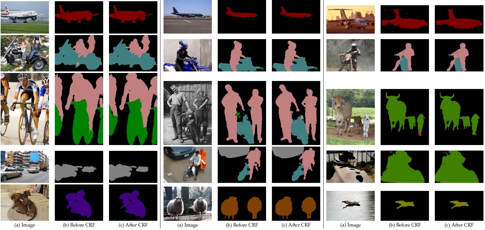
http://liangchiehchen.com/projects/DeepLab.html

SeparableConvolution2D

2次元入力のためのSeparable convolution演算．
Separable convolutionは depth_multiplierは，深さごとの単位で入力チャンネルに対してどれだけ出力チャンネルを生成するかを制御する．直感的には，separable畳み込みは，畳み込みカーネルをより小さい2つのカーネルへ分解かInceptionブロックの極端なものとして理解できる．

Deconvolution2D

transposed convolution = 転置畳み込み。元となる特徴マップを拡大してから畳み込む。

http://qiita.com/shngt/items/9c86e69e16ce6d61a0c6

# apply a 3x3 transposed convolution with stride 1x1 and 3 output filters on a 12x12 image:
model = Sequential()
model.add(Deconvolution2D(3, 3, 3, output_shape=(None, 3, 14, 14), border_mode='valid', input_shape=(3, 12, 12)))
# output_shape will be (None, 3, 14, 14)

# apply a 3x3 transposed convolution with stride 2x2 and 3 output filters on a 12x12 image:
model = Sequential()
model.add(Deconvolution2D(3, 3, 3, output_shape=(None, 3, 25, 25), subsample=(2, 2), border_mode='valid', input_shape=(3, 12, 12)))
model.summary()
# output_shape will be (None, 3, 25, 25)

Convolution3D

3次元入力をフィルターする畳み込み演算．

UpSampling1D

時間軸方向にそれぞれの時間ステップをlength回繰り返す．

UpSampling2D

データの行と列をそれぞれsize[0]及びsize[1]回繰り返す．

UpSampling3D

データの1番目，2番目，3番目の次元をそれぞれsize[0]，size[1]，size[2]だけ繰り返す．

ZeroPadding1D

一次元入力（例，時系列）に対するゼロパディングレイヤー．

ZeroPadding2D

2次元入力（例，画像）のためのゼロパディングレイヤー

ZeroPadding3D

3次元データ（空間及び時空間）のためのゼロパディングレイヤー．

Poolingレイヤー

MaxPooling1D

時系列データのマックスプーリング演算．

        layer_test(convolutional.MaxPooling1D,
                   kwargs={'stride': 1,
                           'border_mode': 'valid'},
                   input_shape=(3, 5, 4))

MaxPooling2D

空間データのマックスプーリング演算

        layer_test(convolutional.MaxPooling2D,
                   kwargs={'strides': 1,
                           'border_mode': 'valid',
                           'pool_size': pool_size},
                   input_shape=(3, 11, 12, 4))

MaxPooling3D

3次元データ（空間もしくは時空間）に対するマックスプーリング演算．

AveragePooling1D

時系列データのための平均プーリング演算．

AveragePooling2D

空間データのための平均プーリング演算．

AveragePooling3D

3次元データ（空間もしくは時空間）に対する平均プーリング演算．

GlobalMaxPooling1D

時系列データのためのグルーバルなマックスプーリング演算．

GlobalAveragePooling1D

時系列データのためのグルーバルな平均プーリング演算．

GlobalMaxPooling2D

空間データのグルーバルなマックスプーリング演算．

GlobalAveragePooling2D

空間データのグルーバルな平均プーリング演算．

Locally-connectedレイヤー

LocallyConnected1D

重みが共有されないこと，すなわち，異なるフィルタの集合が異なる入力のパッチに適用されること，以外はLocallyConnected1DはConvolution1Dと似たように動作します．
一体何に使うのだと思ったが、実験に使われるそう。人間の単純細胞と複雑細胞では重み共有をしてないそうで、そこを同じにしたいことがあるらしい。

# apply a unshared weight convolution 1d of length 3 to a sequence with
# 10 timesteps, with 64 output filters
model = Sequential()
model.add(LocallyConnected1D(64, 3, input_shape=(10, 32)))
# now model.output_shape == (None, 8, 64)
# add a new conv1d on top
model.add(LocallyConnected1D(32, 3))
# now model.output_shape == (None, 6, 32)

LocallyConnected2D

重みが共有されないこと，すなわち，異なるフィルタの集合が異なる入力のパッチに適用されること，以外はLocallyConnected2DはConvolution2Dと似たように動作します．

# apply a 3x3 unshared weights convolution with 64 output filters on a 32x32 image:
model = Sequential()
model.add(LocallyConnected2D(64, 3, 3, input_shape=(3, 32, 32)))
# now model.output_shape == (None, 64, 30, 30)
# notice that this layer will consume (30*30)*(3*3*3*64) + (30*30)*64 parameters

# add a 3x3 unshared weights convolution on top, with 32 output filters:
model.add(LocallyConnected2D(32, 3, 3))
# now model.output_shape == (None, 32, 28, 28)

畳み込みでの注意

画像のサンプル数、画像のチャネル数（白黒画像なら1、RGBのカラー画像なら3など）、画像の縦幅、画像の横幅の４次元テンソルで入力するのが一般的
th（Theano）では(サンプル数, チャネル数, 画像の行数, 画像の列数)
tf（TensorFlow）では（サンプル数, 画像の行数, 画像の列数, チャネル数）
http://aidiary.hatenablog.com/entry/20161120/1479640534

次元が合わない時には手計算が必要な場合もあるかも

Recurrentレイヤー

SimpleRNN

出力が入力にフィードバックされる全結合RNN．

model.add(SimpleRNN(20, return_sequences=False))

GRU

ゲートのあるリカレントユニット

# Sequentialモデルの最初のレイヤーとして
model = Sequential()
model.add(GRU(32, input_dim=64, input_length=10))

model.add(GRU(16))

LSTM

長短期記憶ユニット

# Sequentialモデルの最初のレイヤーとして
model = Sequential()
model.add(LSTM(32, input_shape=(10, 64)))
# ここで model.output_shape == (None, 32)
# 注: `None`はバッチ次元．note: `None` is the batch dimension.

# 以下は同様の意味です:
model = Sequential()
model.add(LSTM(32, input_dim=64, input_length=10))

# 2層目以降のレイヤーに対しては，入力サイズを指定する必要はありません:
model.add(LSTM(16))

Embeddingレイヤー

Embedding

正の整数（インデックス）を固定次元の密ベクトルに変換します．例）[[4], [20]] -> [[0.25, 0.1], [0.6, -0.2]]
モデルの最初のレイヤーのみ。

model = Sequential()
  model.add(Embedding(1000, 64, input_length=10))
  # このモデルは入力として次元が (batch, input_length) である整数行列を取ります．
  # 最大の整数（つまり，単語インデックス）は1000です（語彙数）．
  # ここで，model.output_shape == (None, 10, 64) となります．Noneはバッチ次元です．

  input_array = np.random.randint(1000, size=(32, 10))

  model.compile('rmsprop', 'mse')
  output_array = model.predict(input_array)
  assert output_array.shape == (32, 10, 64)

Advanced Activationsレイヤー

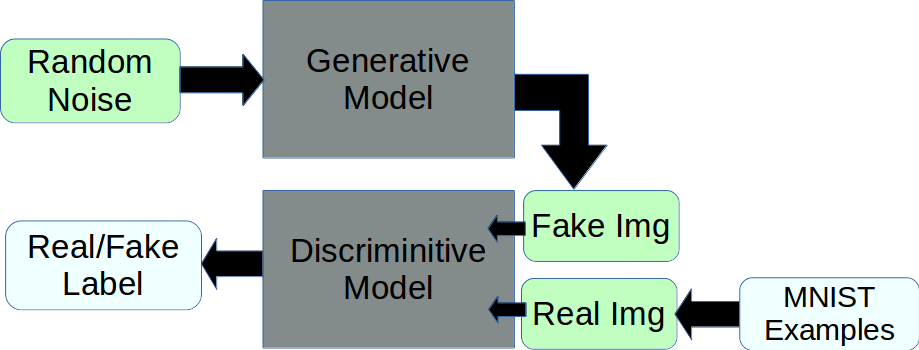
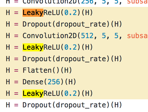
LeakyReLU

ユニットがアクティブでないときに微少な勾配を可能とするRectified Linear Unitの特別なバージョン．

generative adversarial networks (GANs)

PReLU

Parametric Recitied Linear Unit(PReLU)という従来のユニット正規化（整流?）を一般化した手法を提案
PReLUは計算コストの増加をほぼゼロに抑えつつ、モデルのフィッティングと過学習のリスクを改善
非線形な正規化を考慮した頑健な初期化手法を示した
特定のデータセットに対する識別精度で人間(誤認識5.1%)を上回った
http://qiita.com/shima_x/items/8a2f001621dfcbdac028

chainer版
https://github.com/nutszebra/prelu_net

使い方

    from keras.layers.advanced_activations import PReLU
    layer_test(PReLU, kwargs={},
               input_shape=(2, 3, 4))

ELU

Bias Shiftを軽減するために、負の値を取るようにした
・非活性領域でNoiseにRobustになるように、一定の値でSaturationするようにした
・正の領域では入力の大きさによって出力が変わるようにし、負の領域では値の大きさは重要ではないので一定値でSaturationさせる
http://qiita.com/supersaiakujin/items/aec98d0e956d9c815360

    from keras.layers.advanced_activations import ELU
    for alpha in [0., .5, -1.]:
        layer_test(ELU, kwargs={'alpha': alpha},
                   input_shape=(2, 3, 4))

ParametricSoftplus

    from keras.layers.advanced_activations import ParametricSoftplus
    layer_test(ParametricSoftplus,
               kwargs={'alpha_init': 1.,
                       'beta_init': -1},
               input_shape=(2, 3, 4))

ThresholdedReLU

for cl in conv_layers:
    x = Convolution1D(cl[0], cl[1])(x)
    x = ThresholdedReLU(th)(x)
    if not cl[2] is None:
        x = MaxPooling1D(cl[2])(x)

SReLU

    from keras.layers.advanced_activations import SReLU
    layer_test(SReLU, kwargs={},
               input_shape=(2, 3, 4))

BatchNormalization

各バッチ毎に前の層の出力（このレイヤーへの入力）を正規化します．つまり，平均を0，標準偏差を1に近づけるような変換を適用します．
modeは0，1または2の整数。1: sample-wise正規化．このモードは2次元の入力を想定。

models_GAN.py

from keras.layers.normalization import BatchNormalization 
x = Dense(f * start_dim * start_dim, input_dim=noise_dim)(gen_input)
    x = Reshape(reshape_shape)(x)
    x = BatchNormalization(mode=bn_mode, axis=bn_axis)(x)
    x = Activation("relu")(x)

    # Upscaling blocks
    for i in range(nb_upconv):
        x = UpSampling2D(size=(2, 2))(x)
        nb_filters = int(f / (2 ** (i + 1)))
        x = Convolution2D(nb_filters, 3, 3, border_mode="same")(x)
        x = BatchNormalization(mode=bn_mode, axis=1)(x)
        x = Activation("relu")(x)
        x = Convolution2D(nb_filters, 3, 3, border_mode="same")(x)
        x = Activation("relu")(x)

Noiseレイヤー

GaussianNoise

入力に平均0，標準偏差sigmaのガウシアンノイズを加えます。これはオーバーフィッティングの低減に有効です(random data augmentationの一種)。ガウシアンノイズは入力が実数値のときのノイズ付与として一般的です。

    layer_test(noise.GaussianNoise,
               kwargs={'sigma': 1.},
               input_shape=(3, 2, 3))

GaussianDropout

入力に平均1，標準偏差sqrt(p/(1-p))のガウシアンノイズを乗じます。

    layer_test(noise.GaussianDropout,
               kwargs={'p': 0.5},
               input_shape=(3, 2, 3))

レイヤーラッパー: TimeDistributed

入力のすべての時間スライスにレイヤーを適用。
入力は少なくとも3次元である必要があります．インデックスの次元は時間次元であると見なされます．

例えば，32個のサンプルを持つバッチを考えます．各サンプルは16次元で構成される10個のベクトルを持ちます．このとき，バッチの入力の形状は(32, 10, 16)となります（input_shapeはサンプル数の次元を含まないため，(10, 16)となります）．

このとき，10個のタイムスタンプのレイヤーそれぞれにDenseを適用するために，TimeDistributedを利用することができます:

# as the first layer in a model
model = Sequential()
model.add(TimeDistributed(Dense(8), input_shape=(10, 16)))
# now model.output_shape == (None, 10, 8)

# subsequent layers: no need for input_shape
model.add(TimeDistributed(Dense(32)))
# now model.output_shape == (None, 10, 32)

TimeDistributedレイヤを使ってシーケンスタギングフレームワークを実装したいと思います。タスクは、質問をタイムラインに沿った回答のスレッドと照合することです。
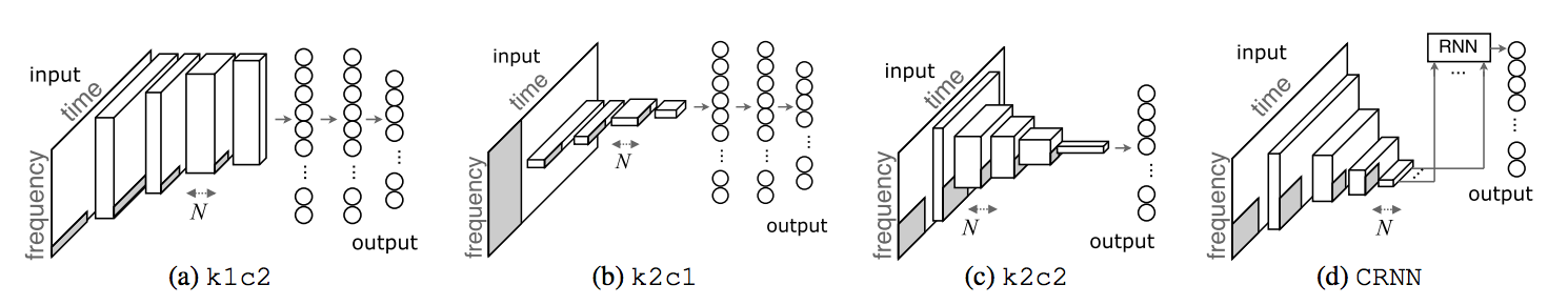
私はLSTMレイヤーを使用して、各タイムステップの入力として、2つのCNN（質問と回答のそれぞれのため）のマージを使ってタイムラインをモデル化します。簡単な図は次のとおりです。

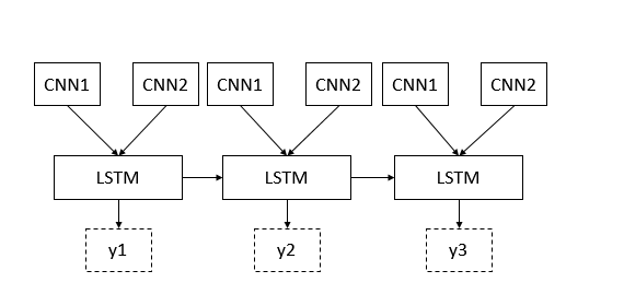
実装では、埋め込みレイヤーを使用して、埋め込みレイヤーを使用して、事前に作成された単語埋め込みを入力シェイプ（1、maxlen_doc、maxlen_sent）に含めました。つまり、最大がmaxlen_doc。
各質問の下の答えと文中の最大単語数はmaxlen_sentです。

model_q = Sequential()
    model_q.add(TimeDistributed(Embedding(input_dim=n_symbols, output_dim=embedding_dim, weights=[pretrained_embeddings]), batch_input_shape=(1, maxlen_doc, maxlen_sent),  input_dtype='int32'))
    model_q.add(Reshape((maxlen_doc, 1, maxlen_sent, embedding_dim)))
    model_q.add(TimeDistributed(Convolution2D(nb_filter=nb_filter1, nb_row=filter_length1, nb_col=embedding_dim, input_shape=(maxlen_doc, 1, maxlen_sent, embedding_dim), border_mode='valid', activation='relu')))
    model_q.add(TimeDistributed(MaxPooling2D(pool_size=(maxlen_sent-filter_length1+1, 1), border_mode='valid')))
    model_q.add(TimeDistributed(Flatten()))

    model_a = Sequential()
    model_a.add(TimeDistributed(Embedding(input_dim=n_symbols, output_dim=embedding_dim, weights=[pretrained_embeddings]), batch_input_shape=(1, maxlen_doc, maxlen_sent),  input_dtype='int32'))
    model_a.add(Reshape((maxlen_doc, 1, maxlen_sent, embedding_dim)))
    model_a.add(TimeDistributed(Convolution2D(nb_filter=nb_filter1, nb_row=filter_length1, nb_col=embedding_dim, input_shape=(maxlen_doc, 1, maxlen_sent, embedding_dim), border_mode='valid', activation='relu')))
    model_a.add(TimeDistributed(MaxPooling2D(pool_size=(maxlen_sent-filter_length1+1, 1), border_mode='valid')))
    model_a.add(TimeDistributed(Flatten()))

    model = Sequential()
    model.add(TimeDistributed(Merge([model_q, model_a], mode='concat', concat_axis=1)))
    model.add(LSTM(output_dim=lstm_output_size, return_sequences=True))
    model.add(Dropout(0.1))
    model.add(TimeDistributed(Dense(100, activation='relu')))
    model.add(TimeDistributed(Dense(3, activation='softmax')))

参考
https://groups.google.com/forum/#!topic/keras-users/dqT2KR59gM0

kerasで強化学習

def custom_Q_nn(agent, env, dropout=0, h0_width=8, h1_width=8, **args):
    S = Input(shape=[agent.input_dim])
    h = Reshape([agent.nframes, agent.input_dim/agent.nframes])(S)
    h = TimeDistributed(Dense(h0_width, activation='relu', init='he_normal'))(h)
    h = Dropout(dropout)(h)
    h = LSTM(h1_width, return_sequences=True)(h)
    h = Dropout(dropout)(h)
    h = LSTM(h1_width)(h)
    h = Dropout(dropout)(h)
    V = Dense(env.action_space.n, activation='linear',init='zero')(h)
    model = Model(S,V)
    model.compile(loss='mse', optimizer=RMSprop(lr=0.01) )
    return model

agent = keras.agents.D2QN(env, modelfactory=custom_Q_nn)

オリジナルのKerasレイヤーを作成する

シンプルで状態を持たない独自演算では、layers.core.Lambdaを用いるべきでしょう。しかし、学習可能な重みを持つような独自演算は、自身でレイヤーを実装する必要があります。

from keras import backend as K
from keras.engine.topology import Layer
import numpy as np

class MyLayer(Layer):
    def __init__(self, output_dim, **kwargs):
        self.output_dim = output_dim
        super(MyLayer, self).__init__(**kwargs)

    def build(self, input_shape):
        input_dim = input_shape[1]
        initial_weight_value = np.random.random((input_dim, output_dim))
        self.W = K.variable(initial_weight_value)
        self.trainable_weights = [self.W]

    def call(self, x, mask=None):
        return K.dot(x, self.W)

    def get_output_shape_for(self, input_shape):
        return (input_shape[0], self.output_dim)

build(input_shape): これは重みを定義するメソッドです。学習可能な重みはリストself.trainable_weightsに追加されます。他の注意すべき属性は以下の通りです。self.updates(更新されるタプル(tensor, new_tensor)のリスト)。non_trainable_weightsとupdatesの使用例は、BatchNormalizationレイヤーのコードを参照してください。
call(x): ここではレイヤーのロジックを記述します。オリジナルのレイヤーでマスキングをサポートしない限り、第一引数の入力テンソルがcallに渡されることに気を付けてください。
get_output_shape_for(input_shape): 作成したレイヤーの内部で入力の形状を変更する場合には、ここで形状変換のロジックを指定する必要があります。こうすることでKerasは、自動的に形状を推定できます。

全結合層(Dense)を見て見る

重みを定義。

class Dense(Layer):
    def build(self, input_shape):
        assert len(input_shape) >= 2
        input_dim = input_shape[-1]
        self.input_dim = input_dim
        self.input_spec = [InputSpec(dtype=K.floatx(),
                                     ndim='2+')]

        self.W = self.add_weight((input_dim, self.output_dim),
                                 initializer=self.init,
                                 name='{}_W'.format(self.name),
                                 regularizer=self.W_regularizer,
                                 constraint=self.W_constraint)
        if self.bias:
            self.b = self.add_weight((self.output_dim,),
                                     initializer='zero',
                                     name='{}_b'.format(self.name),
                                     regularizer=self.b_regularizer,
                                     constraint=self.b_constraint)
        else:
            self.b = None

        if self.initial_weights is not None:
            self.set_weights(self.initial_weights)
            del self.initial_weights
        self.built = True

レイヤーのロジックを記述

    def call(self, x, mask=None):
        output = K.dot(x, self.W)
        if self.bias:
            output += self.b
        return self.activation(output)

作成したレイヤーの内部で入力の形状を変換

    def get_output_shape_for(self, input_shape):
        assert input_shape and len(input_shape) >= 2
        assert input_shape[-1] and input_shape[-1] == self.input_dim
        output_shape = list(input_shape)
        output_shape[-1] = self.output_dim
        return tuple(output_shape)

STFT_layer

データの前処理

シーケンスの前処理

pad_sequences

https://hogehuga.com/post-1464/
2次元のNumpy配列に変換
maxlenを５に指定すると長さ５の配列に膨らまされたり、切り詰められたりする。
’he is poop’　は　[0,0,8,6,9]など。

skipgrams

単語インデックスのシーケンス（整数のリスト）を以下の2つの形式に変換します:

(word, word in the same window), with label 1 (positive samples).
(word, random word from the vocabulary), with label 0 (negative samples).

make_sampling_table

skipgramsのsampling_table引数を生成するために利用します．sampling_table[i]はデータセット中でi番目に頻出する単語をサンプリングする確率です（バランスを保つために，より頻出する語はこれより低い頻度でサンプリングされます）．

テキストの前処理

text_to_word_sequence

文章を単語のリストに分割します．

one_hot

文章を単語インデックス（語彙数n）のリストに1-hotエンコード

Tokenizer

テキストをベクトル化する，または／かつ，テキストをシーケンス（= データセット中でランクi（1から始まる）の単語がインデックスiを持つ単語インデックスのリスト）に変換するクラス．

ImageDataGenerator (画像データジェネレータ)

リアルタイムにデータ拡張しながら，テンソル画像データのバッチを生成します．また，このジェネレータは，データを無限にループするので，無限にバッチを生成します．

datagen = ImageDataGenerator(rotation_range=90)

目的関数の利用方法

model.compile(loss='mean_squared_error', optimizer='sgd')

最適化

SGD,RMSprop,Adagrad,Adadelta,Adam,Adamax,Nadam

sgd = SGD(lr=0.01, clipvalue=0.5)

活性化関数

softmax

softmax 3d 4dの場合
https://github.com/fchollet/keras/blob/master/keras/activations.py#L25
https://github.com/fchollet/keras/issues/5064

tensorflowのv1以上だとndimを増やせば大丈夫な実装が入ってる

ndim = K.ndim(x)
    if ndim == 2:
        return K.softmax(x)
    elif ndim > 2:
        e = K.exp(x - K.max(x, axis=axis, keepdims=True))
        s = K.sum(e, axis=axis, keepdims=True)
        return e / s
    else:
        raise ValueError('Cannot apply softmax to a tensor that is 1D')

softplus
softsign
relu
tanh
sigmoid
hard_sigmoid
linear

model.add(Dense(64, activation='tanh'))

コールバック

トレーニング中にモデル内部の状態と統計を可視化する際に、コールバックを使用。chainerやpytorchでいう所のフック。
Sequentialモデルの.fit()メソッドに(キーワード引数callbacksとして)コールバックのリストを渡す。

ModelCheckpoint

全エポック終了後にモデルを保存

EarlyStopping

監視されているデータの変化が停止した時にトレーニングを終了

RemoteMonitor

サーバーにイベントをストリームするときに使用

LearningRateScheduler

学習率を変えるスケジューラ

TensorBoard

Tensorboardによる基本的な可視化。

ReduceLROnPlateau

評価関数の改善が止まった時に学習率を減らす。

CSVLogger

各エポックの結果をcsvファイルに保存するコールバック

LambdaCallback

シンプルな自作コールバックを急いで作るためのコールバック

on_epoch_begin: すべてのエポックの開始時に呼ばれます．
on_epoch_end: すべてのエポックの終了時に呼ばれます．
on_batch_begin: すべてのバッチの開始時に呼ばれます．
on_batch_end: すべてのバッチの終了時に呼ばれます．
on_train_begin: 学習の開始時に呼ばれます．
on_train_end: 学習の終了時に呼ばれます．

# すべてのバッチの開始時にバッチ番号を表示
batch_print_callback = LambdaCallback(on_batch_begin=lambda batch, logs: print(batch))

# すべてのエポックの終了時に損失をプロット
import numpy as np
import matplotlib.pyplot as plt
plot_loss_callback = LambdaCallback(on_epoch_end=lambda epoch, logs: plt.plot(np.arange(epoch), logs['loss']))

# 学習の終了時にいくつかのプロセスを終了
processes = ...
cleanup_callback = LambdaCallback(on_train_end=lambda logs: [p.terminate() for p in processes if p.is_alive()])

model.fit(..., callbacks=[batch_print_callback, plot_loss_callback, cleanup_callback])

lambdaコールバックサンプル
https://github.com/keunwoochoi/keras_callbacks_example

コード詳細がまとまってる
http://qiita.com/yukiB/items/f45f0f71bc9739830002

データセット

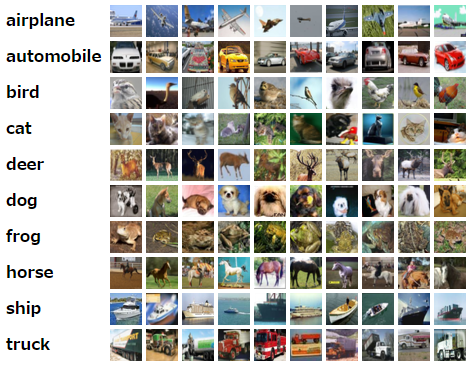
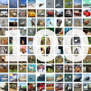
CIFAR10 画像分類

10のクラスにラベル付けされた、50000枚の32x32訓練用カラー画像、10000枚のテスト用画像のデータセット。

from keras.datasets import cifar10

(X_train, y_train), (X_test, y_test) = cifar10.load_data()

CIFAR100 画像分類

100のクラスにラベル付けされた、50000枚の32x32訓練用カラー画像、10000枚のテスト用画像のデータセット。

from keras.datasets import cifar100

(X_train, y_train), (X_test, y_test) = cifar100.load_data(label_mode='fine')

IMDB映画レビュー感情分類

感情(肯定/否定)のラベル付けをされた、25,000のIMDB映画レビューのデータセット。

from keras.datasets import imdb

(X_train, y_train), (X_test, y_test) = imdb.load_data(path="imdb_full.pkl",
                                                      nb_words=None,
                                                      skip_top=0,
                                                      maxlen=None,
                                                      seed=113,
                                                      start_char=1,
                                                      oov_char=2,
                                                      index_from=3)

ロイターのニュースワイヤートピックス分類

46のトピックにラベル付けされた、11,228個のロイターのニュースワイヤーのデータセット。

from keras.datasets import reuters

(X_train, y_train), (X_test, y_test) = reuters.load_data(path="reuters.pkl",
                                                         nb_words=None,
                                                         skip_top=0,
                                                         maxlen=None,
                                                         test_split=0.2,
                                                         seed=113,
                                                         start_char=1,
                                                         oov_char=2,
                                                         index_from=3)

MNIST 手書き数字データベース

60,000枚の28x28、10個の数字の白黒画像と10,000枚のテスト用画像データセット。

from keras.datasets import mnist

(X_train, y_train), (X_test, y_test) = mnist.load_data()

Applications

画像分類モデルの使用例

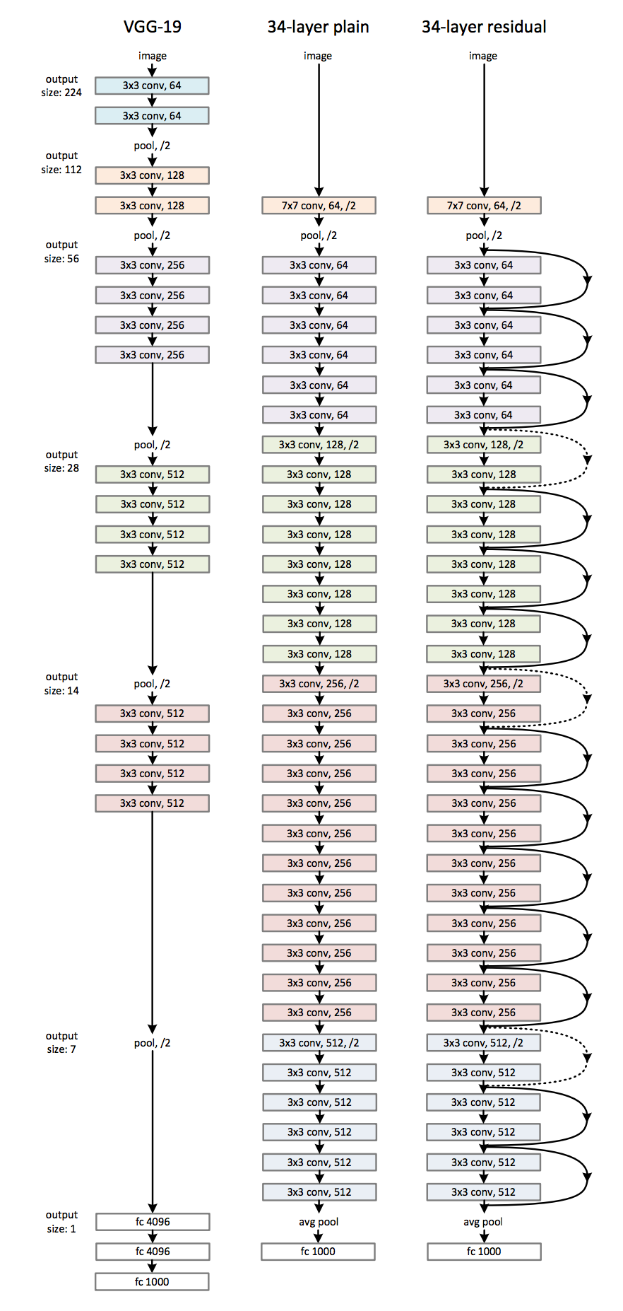
Xception
VGG16
VGG19
ResNet50
InceptionV3

VGG16

from keras.applications.vgg16 import VGG16
from keras.preprocessing import image
from keras.applications.vgg16 import preprocess_input
import numpy as np

model = VGG16(weights='imagenet', include_top=False)

img_path = 'elephant.jpg'
img = image.load_img(img_path, target_size=(224, 224))
x = image.img_to_array(img)
x = np.expand_dims(x, axis=0)
x = preprocess_input(x)

features = model.predict(x)

VGG19

from keras.applications.vgg19 import VGG19
from keras.preprocessing import image
from keras.applications.vgg19 import preprocess_input
from keras.models import Model
import numpy as np

base_model = VGG19(weights='imagenet')
model = Model(input=base_model.input, output=base_model.get_layer('block4_pool').output)

img_path = 'elephant.jpg'
img = image.load_img(img_path, target_size=(224, 224))
x = image.img_to_array(img)
x = np.expand_dims(x, axis=0)
x = preprocess_input(x)

block4_pool_features = model.predict(x)

ResNet50

from keras.applications.resnet50 import ResNet50
from keras.preprocessing import image
from keras.applications.resnet50 import preprocess_input, decode_predictions
import numpy as np

model = ResNet50(weights='imagenet')

img_path = 'elephant.jpg'
img = image.load_img(img_path, target_size=(224, 224))
x = image.img_to_array(img)
x = np.expand_dims(x, axis=0)
x = preprocess_input(x)

preds = model.predict(x)
# decode the results into a list of tuples (class, description, probability)
# (one such list for each sample in the batch)
print('Predicted:', decode_predictions(preds, top=3)[0])
# Predicted: [(u'n02504013', u'Indian_elephant', 0.82658225), (u'n01871265', u'tusker', 0.1122357), (u'n02504458', u'African_elephant', 0.061040461)]

InceptionV3

from keras.applications.inception_v3 import InceptionV3
from keras.preprocessing import image
from keras.models import Model
from keras.layers import Dense, GlobalAveragePooling2D
from keras import backend as K

# create the base pre-trained model
base_model = InceptionV3(weights='imagenet', include_top=False)

# add a global spatial average pooling layer
x = base_model.output
x = GlobalAveragePooling2D()(x)
# let's add a fully-connected layer
x = Dense(1024, activation='relu')(x)
# and a logistic layer -- let's say we have 200 classes
predictions = Dense(200, activation='softmax')(x)

# this is the model we will train
model = Model(input=base_model.input, output=predictions)

# first: train only the top layers (which were randomly initialized)
# i.e. freeze all convolutional InceptionV3 layers
for layer in base_model.layers:
    layer.trainable = False

# compile the model (should be done *after* setting layers to non-trainable)
model.compile(optimizer='rmsprop', loss='categorical_crossentropy')

# train the model on the new data for a few epochs
model.fit_generator(...)

# at this point, the top layers are well trained and we can start fine-tuning
# convolutional layers from inception V3. We will freeze the bottom N layers
# and train the remaining top layers.

# let's visualize layer names and layer indices to see how many layers
# we should freeze:
for i, layer in enumerate(base_model.layers):
   print(i, layer.name)

# we chose to train the top 2 inception blocks, i.e. we will freeze
# the first 172 layers and unfreeze the rest:
for layer in model.layers[:172]:
   layer.trainable = False
for layer in model.layers[172:]:
   layer.trainable = True

# we need to recompile the model for these modifications to take effect
# we use SGD with a low learning rate
from keras.optimizers import SGD
model.compile(optimizer=SGD(lr=0.0001, momentum=0.9), loss='categorical_crossentropy')

# we train our model again (this time fine-tuning the top 2 inception blocks
# alongside the top Dense layers
model.fit_generator(...)

MusicTaggerCRNN

ベクトルで表現された楽曲のメルスペクトログラムを入力とし，そのジャンルを出力すconvolutional-recurrentモデル．

from keras.applications.music_tagger_crnn import MusicTaggerCRNN
from keras.applications.music_tagger_crnn import preprocess_input, decode_predictions
import numpy as np

# 1. Tagging
model = MusicTaggerCRNN(weights='msd')

audio_path = 'audio_file.mp3'
melgram = preprocess_input(audio_path)
melgrams = np.expand_dims(melgram, axis=0)

preds = model.predict(melgrams)
print('Predicted:')
print(decode_predictions(preds))
# print: ('Predicted:', [[('rock', 0.097071797), ('pop', 0.042456303), ('alternative', 0.032439161), ('indie', 0.024491295), ('female vocalists', 0.016455274)]])

#. 2. Feature extraction
model = MusicTaggerCRNN(weights='msd', include_top=False)

audio_path = 'audio_file.mp3'
melgram = preprocess_input(audio_path)
melgrams = np.expand_dims(melgram, axis=0)

feats = model.predict(melgrams)
print('Features:')
print(feats[0, :10])
# print: ('Features:', [-0.19160545 0.94259131 -0.9991011 0.47644514 -0.19089699 0.99033844 0.1103896 -0.00340496 0.14823607 0.59856361])

その他
http://josephpcohen.com/w/visualizing-cnn-architectures-side-by-side-with-mxnet/

バックエンド

TheanoバックエンドとTensorFlowバックエンド，が利用可能。

tf.placeholder()やT.matrix(), T.tensor3()をラッピング

from keras import backend as K
input = K.placeholder(shape=(2, 4, 5))
# 以下も動作します:
input = K.placeholder(shape=(None, 4, 5))
# 以下も動作します:
input = K.placeholder(ndim=3)

tf.variable()やtheano.shared()をラッピング

val = np.random.random((3, 4, 5))
var = K.variable(value=val)

# すべて0の変数:
var = K.zeros(shape=(3, 4, 5))
# すべて1の変数:
var = K.ones(shape=(3, 4, 5))

a = b + c * K.abs(d)
c = K.dot(a, K.transpose(b))
a = K.sum(b, axis=2)
a = K.softmax(b)
a = concatenate([b, c], axis=-1)

epsilon
数値演算で使われる微小値を返します．
set_epsilon
数値演算で使われる微小値をセットします．
floatx
デフォルトのfloat型を文字列で返します

詳細
https://keras.io/ja/backend/

初期化

レイヤーの重み初期化方法

uniform
lecun_uniform: input数の平方根でスケーリングした一様分布 (LeCun 98)
normal
identity: shape[0] == shape[1]の2次元のレイヤーで使えます
orthogonal: shape[0] == shape[1]の2次元のレイヤーで使えます
zero
glorot_normal: fan_in + fan_outでスケーリングした正規分布 (Glorot 2010)
glorot_uniform
he_normal: fan_inでスケーリングした正規分布 (He et al., 2014)
he_uniform

model.add(Dense(64, init='uniform'))

from keras import backend as K
import numpy as np

def my_init(shape, name=None):
    value = np.random.random(shape)
    return K.variable(value, name=name)

model.add(Dense(64, init=my_init))

initializations関数を使った場合

from keras import initializations

def my_init(shape, name=None):
    return initializations.normal(shape, scale=0.01, name=name)

model.add(Dense(64, init=my_init))

正則化

レイヤーパラメータあるいはレイヤーの出力に制約を課すことができる。
W_regularizer: keras.regularizers.WeightRegularizer のインスタンス
b_regularizer: keras.regularizers.WeightRegularizer のインスタンス
activity_regularizer: keras.regularizers.ActivityRegularizer のインスタンス

from keras.regularizers import l2, activity_l2
model.add(Dense(64, input_dim=64, W_regularizer=l2(0.01), activity_regularizer=activity_l2(0.01)))

制約

最適化中のネットワークパラメータに制約（例えば非負の制約）を設定することができる。

from keras.constraints import maxnorm
model.add(Dense(64, W_constraint = maxnorm(2)))

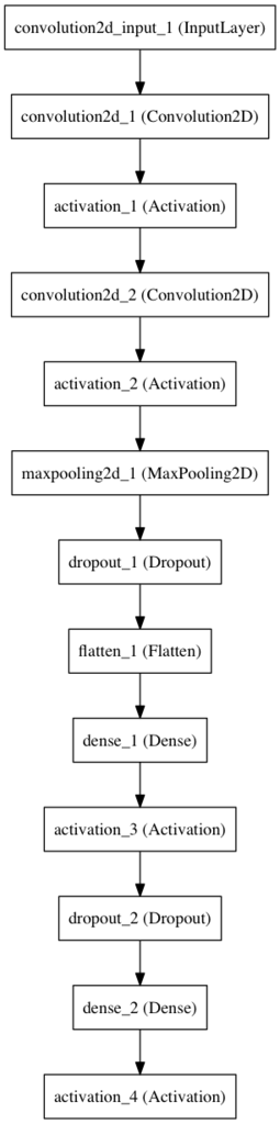
可視化

mac

brew install graphviz

ubuntu

sudo apt-get install graphviz

pip install pydot_ng

from keras.utils.visualize_util import plot
plot(model, to_file='model.png')

Scikit-learn API

KerasのSequentialモデル（1つの入力のみ）をScikit-Learnワークフローの一部として利用することができる。

KerasClassifierの例

from keras.models import Sequential
from keras.layers import Dense
from keras.layers import Dropout
from keras.optimizers import SGD
from keras.wrappers.scikit_learn import KerasClassifier
from sklearn.grid_search import GridSearchCV
import numpy
import pandas
# Function to create model, required for KerasClassifier
def create_model(dropout_rate=0.0):
    # create model
    model = Sequential()
    model.add(Dense(12, input_dim=8, activation='relu'))
    model.add(Dropout(dropout_rate))
    model.add(Dense(8, init='normal', activation='relu'))
    model.add(Dropout(dropout_rate))
    model.add(Dense(1, init='normal', activation='sigmoid'))
    # Compile model
    model.compile(loss='binary_crossentropy', optimizer='adam', metrics=['accuracy'])
    return model

# fix random seed for reproducibility
seed = 7
numpy.random.seed(seed)
# load dataset
dataset = numpy.loadtxt("pima-indians-diabetes.csv", delimiter=",")
# split into input (X) and output (Y) variables
X = dataset[:,0:8]
Y = dataset[:,8]
# create model
model = KerasClassifier(build_fn=create_model, nb_epoch=100, batch_size=5, verbose=0)
# grid search dropout rate
dropout_rate = [0.0, 0.2, 0.5]
param_grid = dict(dropout_rate=dropout_rate)
grid = GridSearchCV(estimator=model, param_grid=param_grid, cv=5)
grid_result = grid.fit(X, Y)
# summarize results
print("Best: %f using %s" % (grid_result.best_score_, grid_result.best_params_))
for params, mean_score, scores in grid_result.grid_scores_:
    print("%f (%f) with: %r" % (scores.mean(), scores.std(), params))

Scikit-learnでハイパーパラメータのグリッドサーチ

# -*- coding: utf-8 -*-

from sklearn import datasets
from sklearn.cross_validation import train_test_split
from sklearn.grid_search import GridSearchCV
from sklearn.metrics import classification_report, confusion_matrix
from sklearn.svm import SVC

## データの読み込み
digits = datasets.load_digits()
X = digits.data
y = digits.target

## トレーニングデータとテストデータに分割．
X_train, X_test, y_train, y_test = train_test_split(
    X, y, test_size=0.5, random_state=0)

## チューニングパラメータ
tuned_parameters = [{'kernel': ['rbf'], 'gamma': [1e-3, 1e-4],
                     'C': [1, 10, 100, 1000]},
                    {'kernel': ['linear'], 'C': [1, 10, 100, 1000]}]

scores = ['accuracy', 'precision', 'recall']

for score in scores:
    print '\n' + '='*50
    print score
    print '='*50

    clf = GridSearchCV(SVC(C=1), tuned_parameters, cv=5, scoring=score, n_jobs=-1)
    clf.fit(X_train, y_train)

    print "\n+ ベストパラメータ:\n"
    print clf.best_estimator_

    print"\n+ トレーニングデータでCVした時の平均スコア:\n"
    for params, mean_score, all_scores in clf.grid_scores_:
        print "{:.3f} (+/- {:.3f}) for {}".format(mean_score, all_scores.std() / 2, params)

    print "\n+ テストデータでの識別結果:\n"
    y_true, y_pred = y_test, clf.predict(X_test)
    print classification_report(y_true, y_pred)

Keras with GridSearchCVでパラメータ最適化自動化

import numpy as np
from sklearn import datasets, preprocessing
from sklearn.model_selection import train_test_split
from sklearn.model_selection import GridSearchCV
from keras.models import Sequential
from keras.layers.core import Dense, Activation
from keras.utils import np_utils
from keras import backend as K
from keras.wrappers.scikit_learn import KerasClassifier


# import data and divided it into training and test purposes
iris = datasets.load_iris()
x = preprocessing.scale(iris.data)
y = np_utils.to_categorical(iris.target)
x_tr, x_te, y_tr, y_te = train_test_split(x, y, train_size  = 0.7)
num_classes = y_te.shape[1]


# Define model for iris classification
def iris_model(activation="relu", optimizer="adam", out_dim=100):
    model = Sequential()
    model.add(Dense(out_dim, input_dim=4, activation=activation))
    model.add(Dense(out_dim, activation=activation))   
    model.add(Dense(num_classes, activation="softmax"))
    model.compile(loss='categorical_crossentropy', optimizer=optimizer, metrics=['accuracy'])
    return model

# Define options for parameters
activation = ["relu", "sigmoid"]
optimizer = ["adam", "adagrad"]
out_dim = [100, 200]
nb_epoch = [10, 25]
batch_size = [5, 10]


# Retrieve model and parameter into GridSearchCV
model = KerasClassifier(build_fn=iris_model, verbose=0)
param_grid = dict(activation=activation, 
                  optimizer=optimizer, 
                  out_dim=out_dim, 
                  nb_epoch=nb_epoch, 
                  batch_size=batch_size)
grid = GridSearchCV(estimator=model, param_grid=param_grid)


# Run grid search
grid_result = grid.fit(x_tr, y_tr)


# Get the best score and the optimized mode
print (grid_result.best_score_)
print (grid_result.best_params_)

# Evaluate the model with test data
grid_eval = grid.predict(x_te)
def y_binary(i):
    if   i == 0: return [1, 0, 0]
    elif i == 1: return [0, 1, 0]
    elif i == 2: return [0, 0, 1]
y_eval = np.array([y_binary(i) for i in grid_eval])
accuracy = (y_eval == y_te)
print (np.count_nonzero(accuracy == True) / (accuracy.shape[0] * accuracy.shape[1]))


# Now see the optimized model
model = iris_model(activation=grid_result.best_params_['activation'], 
                   optimizer=grid_result.best_params_['optimizer'], 
                   out_dim=grid_result.best_params_['out_dim'])
model.summary()

ユーティリティ

データユーティリティ

get_file

既にキャッシュされていないならURLからファイルをダウンロードします。

include_top: ネットワークの出力層側にある3つの全結合層を含むかどうか．

def VGG19(include_top=True, weights='imagenet',
          input_tensor=None):
    '''Instantiate the VGG19 architecture,
    optionally loading weights pre-trained
    on ImageNet. Note that when using TensorFlow,
    for best performance you should set
    `image_dim_ordering="tf"` in your Keras config
    at ~/.keras/keras.json.

    The model and the weights are compatible with both
    TensorFlow and Theano. The dimension ordering
    convention used by the model is the one
    specified in your Keras config file.

    # Arguments
        include_top: whether to include the 3 fully-connected
            layers at the top of the network.
        weights: one of `None` (random initialization)
            or "imagenet" (pre-training on ImageNet).
        input_tensor: optional Keras tensor (i.e. output of `layers.Input()`)
            to use as image input for the model.

    # Returns
        A Keras model instance.
    '''
    if weights not in {'imagenet', None}:
        raise ValueError('The `weights` argument should be either '
                         '`None` (random initialization) or `imagenet` '
                         '(pre-training on ImageNet).')
    # Determine proper input shape
    if K.image_dim_ordering() == 'th':
        if include_top:
            input_shape = (3, 224, 224)
        else:
            input_shape = (3, None, None)
    else:
        if include_top:
            input_shape = (224, 224, 3)
        else:
            input_shape = (None, None, 3)

    if input_tensor is None:
        img_input = Input(shape=input_shape)
    else:
        if not K.is_keras_tensor(input_tensor):
            img_input = Input(tensor=input_tensor)
        else:
            img_input = input_tensor
    # Block 1
    x = Convolution2D(64, 3, 3, activation='relu', border_mode='same', name='block1_conv1')(img_input)
    x = Convolution2D(64, 3, 3, activation='relu', border_mode='same', name='block1_conv2')(x)
    x = MaxPooling2D((2, 2), strides=(2, 2), name='block1_pool')(x)

    # Block 2
    x = Convolution2D(128, 3, 3, activation='relu', border_mode='same', name='block2_conv1')(x)
    x = Convolution2D(128, 3, 3, activation='relu', border_mode='same', name='block2_conv2')(x)
    x = MaxPooling2D((2, 2), strides=(2, 2), name='block2_pool')(x)

    # Block 3
    x = Convolution2D(256, 3, 3, activation='relu', border_mode='same', name='block3_conv1')(x)
    x = Convolution2D(256, 3, 3, activation='relu', border_mode='same', name='block3_conv2')(x)
    x = Convolution2D(256, 3, 3, activation='relu', border_mode='same', name='block3_conv3')(x)
    x = Convolution2D(256, 3, 3, activation='relu', border_mode='same', name='block3_conv4')(x)
    x = MaxPooling2D((2, 2), strides=(2, 2), name='block3_pool')(x)

    # Block 4
    x = Convolution2D(512, 3, 3, activation='relu', border_mode='same', name='block4_conv1')(x)
    x = Convolution2D(512, 3, 3, activation='relu', border_mode='same', name='block4_conv2')(x)
    x = Convolution2D(512, 3, 3, activation='relu', border_mode='same', name='block4_conv3')(x)
    x = Convolution2D(512, 3, 3, activation='relu', border_mode='same', name='block4_conv4')(x)
    x = MaxPooling2D((2, 2), strides=(2, 2), name='block4_pool')(x)

    # Block 5
    x = Convolution2D(512, 3, 3, activation='relu', border_mode='same', name='block5_conv1')(x)
    x = Convolution2D(512, 3, 3, activation='relu', border_mode='same', name='block5_conv2')(x)
    x = Convolution2D(512, 3, 3, activation='relu', border_mode='same', name='block5_conv3')(x)
    x = Convolution2D(512, 3, 3, activation='relu', border_mode='same', name='block5_conv4')(x)
    x = MaxPooling2D((2, 2), strides=(2, 2), name='block5_pool')(x)

    if include_top:
        # Classification block
        x = Flatten(name='flatten')(x)
        x = Dense(4096, activation='relu', name='fc1')(x)
        x = Dense(4096, activation='relu', name='fc2')(x)
        x = Dense(1000, activation='softmax', name='predictions')(x)

    # Create model
    model = Model(img_input, x)

    # load weights
    if weights == 'imagenet':
        print('K.image_dim_ordering:', K.image_dim_ordering())
        if K.image_dim_ordering() == 'th':
            if include_top:
                weights_path = get_file('vgg19_weights_th_dim_ordering_th_kernels.h5',
                                        TH_WEIGHTS_PATH,
                                        cache_subdir='models')
            else:
                weights_path = get_file('vgg19_weights_th_dim_ordering_th_kernels_notop.h5',
                                        TH_WEIGHTS_PATH_NO_TOP,
                                        cache_subdir='models')
            model.load_weights(weights_path)
            if K.backend() == 'tensorflow':
                warnings.warn('You are using the TensorFlow backend, yet you '
                              'are using the Theano '
                              'image dimension ordering convention '
                              '(`image_dim_ordering="th"`). '
                              'For best performance, set '
                              '`image_dim_ordering="tf"` in '
                              'your Keras config '
                              'at ~/.keras/keras.json.')
                convert_all_kernels_in_model(model)
        else:
            if include_top:
                weights_path = get_file('vgg19_weights_tf_dim_ordering_tf_kernels.h5',
                                        TF_WEIGHTS_PATH,
                                        cache_subdir='models')
            else:
                weights_path = get_file('vgg19_weights_tf_dim_ordering_tf_kernels_notop.h5',
                                        TF_WEIGHTS_PATH_NO_TOP,
                                        cache_subdir='models')
            model.load_weights(weights_path)
            if K.backend() == 'theano':
                convert_all_kernels_in_model(model)
    return model

出入力ユーティリティ

HDF5Matrix

Numpyの配列の代わりに使えるHDF5データセットの表現です．

X_data = HDF5Matrix('input/file.hdf5', 'data')
model.predict(X_data)

startとendを指定することでデータセットをスライスすることができます。

from keras.models import Sequential
from keras.layers import Dense
from keras.utils.io_utils import HDF5Matrix
import numpy as np

def create_dataset():
    import h5py
    X = np.random.randn(200,10).astype('float32')
    y = np.random.randint(0, 2, size=(200,))
    f = h5py.File('test.h5', 'w')
    # Creating dataset to store features
    X_dset = f.create_dataset('my_data', (200,10), dtype='f')
    X_dset[:] = X
    # Creating dataset to store labels
    y_dset = f.create_dataset('my_labels', (200,), dtype='i')
    y_dset[:] = y
    f.close()

create_dataset()

# Instantiating HDF5Matrix for the training set, which is a slice of the first 150 elements
X_train = HDF5Matrix('test.h5', 'my_data', start=0, end=150)
y_train = HDF5Matrix('test.h5', 'my_labels', start=0, end=150)

# Likewise for the test set
X_test = HDF5Matrix('test.h5', 'my_data', start=150, end=200)
y_test = HDF5Matrix('test.h5', 'my_labels', start=150, end=200)

# HDF5Matrix behave more or less like Numpy matrices with regards to indexing
print(y_train[10])
# But they do not support negative indices, so don't try print(X_train[-1])

model = Sequential()
model.add(Dense(64, activation='relu'))
model.add(Dense(1, activation='sigmoid'))

model.compile(loss='binary_crossentropy', optimizer='sgd')

model.fit(X_train, y_train, batch_size=32)

model.evaluate(X_test, y_test, batch_size=32)

レイヤーユーティリティ

layer_from_config

model = load_model('model1.h5')                                                                         
layer1 = model.layers.pop() # Copy activation_6 layer                                      
layer2 = model.layers.pop() # Copy classification layer (dense_2)                          

model.add(Dense(512, name='dense_3'))
model.add(Activation('softmax', name='activation_7'))

# get layer1 config
layer1_config = layer1.get_config()
layer2_config = layer2.get_config()
# change the name of the layers otherwise it complains
layer1_config['name'] = layer1_config['name'] + '_new'
layer2_config['name'] = layer2_config['name'] + '_new'

# import the magic function
from keras.utils.layer_utils import layer_from_config
# re-add new layers from the config of the old ones 
model.add(layer_from_config({'class_name':type(l2), 'config':layer2_config}))
model.add(layer_from_config({'class_name':type(l1), 'config':layer1_config}))

model.compile(...)

print(model.summary())

Numpyユーティリティ

to_categorical

クラスベクトル（0からnb_classesまでの整数）を categorical_crossentropyとともに用いるためのバイナリのクラス行列に変換します．

http://may46onez.hatenablog.com/entry/2016/07/14/122047
Kerasはラベルを数値ではなく、0or1を要素に持つベクトルで扱うらしい
つまりあるサンプルに対するターゲットを「3」だとすると
[0, 0, 0, 1, 0, 0, 0, 0, 0, 0]

from keras.utils import np_utils
y_train = np_utils.to_categorical(y_train)
y_test = np_utils.to_categorical(y_test)

convert_kernel

カーネル行列（Numpyの配列）をTheano形式からTensorFlow形式に変換します。（この変換は逆変換と同一なので，TensorFlow形式からTheano形式への変換も可能です）

converted_w = convert_kernel(original_w)

サンプルコード

文字レベル畳み込みニューラルネットワークを用いたテキスト分類の実装
https://github.com/mhjabreel/CharCnn_Keras
KerasのCNNを使って文書分類する
https://hogehuga.com/post-1464/

kerasのサンプル
https://github.com/fchollet/keras-resources
https://github.com/tdeboissiere/DeepLearningImplementations

keras-rl（強化学習）
https://github.com/matthiasplappert/keras-rl/blob/master/examples/dqn_atari.py

動画

データサイエンスマシンラーニングエッセンシャル
https://www.edx.org/course/data-science-machine-learning-essentials-microsoft-dat203x-0
データ科学入門
https://www.coursera.org/course/datasci
機械学習の紹介
https://www.udacity.com/course/intro-to-machine-learning–ud120
機械学習のニューラルネットワーク
https://www.coursera.org/course/neuralnets
ディープラーニング
https://www.udacity.com/course/deep-learning–ud730
強化学習
https://www.udacity.com/course/reinforcement-learning–ud600

気になるページ

R-cnn
https://github.com/ishay2b/VanillaCNN
http://pjreddie.com/darknet/yolo/
ttps://github.com/rbgirshick/fast-rcnn
https://github.com/rbgirshick/py-faster-rcnn
https://github.com/mitmul/deeppose
https://github.com/shihenw/convolutional-pose-machines-release
https://github.com/anewell/pose-hg-train
http://mscoco.org/

Reinforcement Learning
http://fidoproject.github.io/
https://github.com/sisl/Chimp
https://robosamir.github.io/DDPG-on-a-Real-Robot/
https://github.com/carlos-cardoso/robot-skills
https://vmayoral.github.io/robots,/simulation,/ai,/rl,/reinforcement/learning/2016/08/19/openai-gym-for-robotics/
https://jamh-web.appspot.com/download.htm
https://handong1587.github.io/deep_learning/2015/10/09/dl-and-autonomous-driving.html
http://openrave.org/docs/latest_stable/

keras
http://ben.bolte.cc/blog/2016/keras-language-modeling.html

tensorflow
https://github.com/corrieelston/datalab/blob/master/FinancialTimeSeriesTensorFlow.ipynb