円運動の重ね合わせでお絵かき【フーリエ変換】 #Python

初投稿です。
高校生でもわかるように書いたつもりです。
実装が読みづらいのはご容赦ください。

絵のキャラクターは、.LIVEの神楽すずさん（緑）と、ヤマトイオリさん（水色）です。
本ページの作品は二次創作物です。キャラクターに関する知的財産権は株式会社アップランドに帰属します。

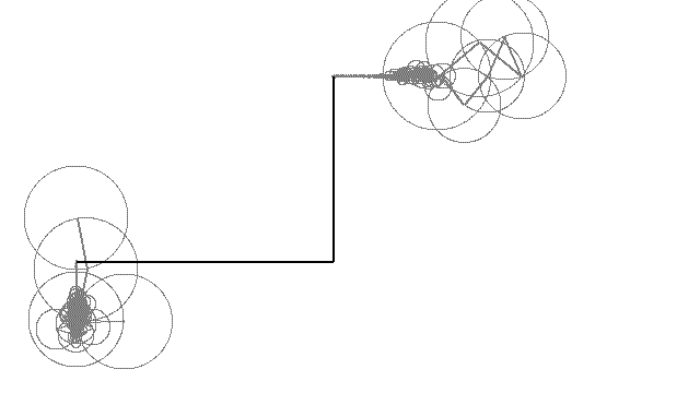
作品例

こういうやつです。

大まかな流れ

結ぶと絵になる順序付きの点の集まりを作る
↓
x座標とy座標をそれぞれ高速フーリエ変換する
↓
円運動の重ね合わせで描ける

環境

macOS Big Sur 11.1
PowerPoint for Mac 16.44
Python 3.7.4
beautifulsoup4 4.8.0
matplotlib 3.1.1 (なくてもできる)
numpy 1.17.2
pillow 6.2.0
tqdm 4.36.1 (なくてもできる）

手順

結ぶと絵になる点の集まりをすでに持っている人は、離散フーリエ変換のところまで飛ばしてください。

PowerPointで絵を描く

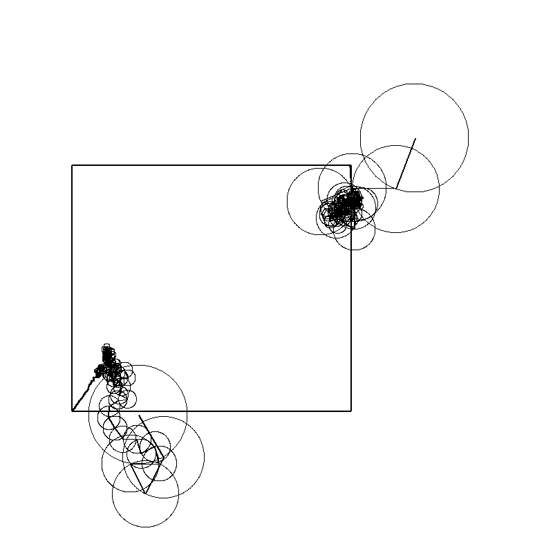
PowerPointの「曲線」で、絵を一筆書きします。
一筆書きというのが、何気に結構難しいです。

.pptxを.zipに書き換えて解凍する

.pptxを.zipに書き換えて解凍すると、以下のようなxmlがでてきます。
正規分布がPowerPointで描画できればいいのにを参考にしました。

解凍したファイル/ppt/slides/slide1.xml

(省略)
<a:pathLst>
    <a:path w="6982104" h="6267205">
        <a:moveTo>
            <a:pt x="2424619" y="3964459"/>
        </a:moveTo>
        <a:cubicBezTo>
            <a:pt x="2459747" y="3967701"/>
            <a:pt x="2494875" y="3970944"/>
            <a:pt x="2534866" y="3945004"/>
        </a:cubicBezTo>
        <a:cubicBezTo>
            <a:pt x="2574858" y="3919064"/>
            <a:pt x="2615930" y="3853132"/>
            <a:pt x="2664568" y="3808817"/>
        </a:cubicBezTo>
        <a:cubicBezTo>
            <a:pt x="2713206" y="3764502"/>
            <a:pt x="2757521" y="3720187"/>
            <a:pt x="2826695" y="3679115"/>
        </a:cubicBezTo>
        <a:cubicBezTo>
(省略)

Cubic Bézier curvesは、4つの点で指定されます。
詳しいことは英語版wikipediaの「Cubic Bézier curves」のところを見てください。
xmlの中身の意味は

xml

(省略)
    <a:pt 1つ目の制御点かつ、ひとつ前の曲線の4つ目の制御点/>
</a:cubicBezTo>
<a:cubicBezTo>
    <a:pt 2つ目の制御点/>
    <a:pt 3つ目の制御点/>
    <a:pt 4つ目の制御点かつ、ひとつ後の曲線の1つ目の制御点/>
</a:cubicBezTo>
(省略)

のようになっているようです。

ベジェ曲線の実装

制御点を、$P_{0}, P_{1}, P_{2}, P_{3}$　として
ベジェ曲線は
$B(t) = (1-t)^{3}P_{0}+3(1-t)^{2}tP_{1}+3(1-t)t^{2}P_{2}+t^{3}P_{3},\quad 0\leq t\leq 1$
と表されます。
そのまま実装しました。

python

import numpy as np

class BezFunc:

    # p は 4つの制御点のリスト
    def __init__(self, p):
        self.p0 = np.array(p[0])
        self.p1 = np.array(p[1])
        self.p2 = np.array(p[2])
        self.p3 = np.array(p[3])

    # 0<=t<=1
    def __call__(self, t):
        return ((1-t)**3)*self.p0+3*((1-t)**2)*t*self.p1+3*(1-t)*(t**2)*self.p2+(t**3)*self.p3

xmlから制御点を抽出して、曲線を描く

xmlから制御点を取り出すにはBeautifulSoupを使います。

python

from bs4 import BeautifulSoup
import numpy as np


class Points:

    def __init__(self, xml_path):
        with open(xml_path, 'r') as f:
            soup = BeautifulSoup(f, 'xml')

        # [[制御点1, 制御点2, 制御点3, 制御点4], [制御点1, 制御点2, …
        bez_points_list = []

        temp_pt = soup.find('a:pathLst').find('a:moveTo').find('a:pt')
        temp_point = (int(temp_pt['x']), int(temp_pt['y']))

        for temp_cubicBezTo in soup.find('a:pathLst').find_all('a:cubicBezTo'):
            temp_list = [temp_point]
            for temp_pt in temp_cubicBezTo.find_all('a:pt'):
                temp_point = (int(temp_pt['x']), int(temp_pt['y']))
                temp_list.append(temp_point)
            bez_points_list.append(temp_list)

        self.bez_points_list = bez_points_list

    # n : 分割数        
    def calc_points(self, n):
        points = []

        for bez_points in self.bez_points_list:
            f = BezFunc(bez_points)
            for i in range(n):
                t = i/n
                points.append(f(t))

        self.points = np.array(points)

    def get_points(self):
        return self.points

使い方

python

xml_path = 'プレゼンテーション/ppt/slides/slide1.xml'
p = Points(xml_path)
p.calc_points(n=5) # 5分割(適当)
points = p.get_points()
points

array([[2424619.   , 3964459.   ], # 1つ目の点の座標
       [2445734.704, 3966170.848], # 2つ目の点の座標
       [2467083.832, 3966482.104], # 3つ目の点の座標
       ...,
       [3557916.696, 5271117.176],
       [3503553.224, 5255947.584],
       [3548753.368, 5184643.528]])

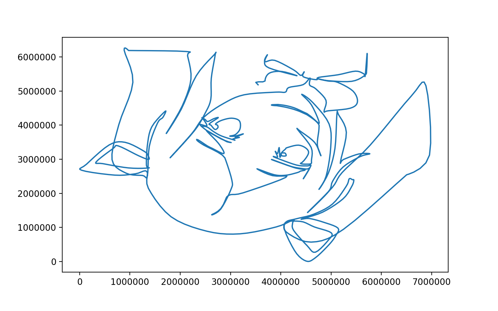
pointsはshape = (点の数, 2)のnumpyの配列です。これを上から順に結んでいけば、絵が描けます。

python

import matplotlib.pyplot as plt

plt.figure(figsize=(8, 5), dpi=200)
plt.plot(points[:,0], points[:,1])
plt.show()

離散フーリエ変換

離散フーリエ変換と逆変換を

F(t) = \sum_{x=0}^{N-1}f(x)e^{-i\frac{2\pi t x}{N}}\\

f(x) = \frac{1}{N}\sum_{t=0}^{N-1}F(t)e^{i\frac{2\pi t x}{N}}

とすると、離散フーリエ変換して逆変換したときに、もとの関数に戻ってきます。
$F(t), \quad f(x)$はそれぞれ、要素がN個の配列だと思ってください。
これは、

離散フーリエ変換

F(t) = \frac{1}{N}\sum_{x=0}^{N-1}f(x)e^{-i\frac{2\pi t x}{N}}\\

f(x) = \sum_{t=0}^{N-1}F(t)e^{i\frac{2\pi t x}{N}}

としても、同じことです。

ここで、

F(t) = A(t)( \cos \phi (t) + i \sin \phi (t))

と表したとき、オイラーの公式

e^{i\theta}=\cos \theta + i \sin \theta

を使うと、逆変換は

\begin{align}
f(x)&= \sum_{t=0}^{N-1}F(t)e^{i\frac{2\pi t x}{N}}\\
&= \sum_{t=0}^{N-1}A(t)( \cos \phi (t) + i \sin \phi (t))(\cos \frac{2\pi t x}{N} + i \sin \frac{2\pi t x}{N})\\
&= \sum_{t=0}^{N-1}A(t)(\cos (\phi (t) +\frac{2\pi t x}{N}) + i \sin (\phi (t) + \frac{2\pi t x}{N}))\\
&= \sum_{t=0}^{N-1}A(t)\cos (\phi (t) +\frac{2\pi t x}{N}) + i \sum_{t=0}^{N-1}A(t) \sin (\phi (t) + \frac{2\pi t x}{N})\\

\end{align}

となり、$f(x)$を実数とすると、第2項はゼロになるので、

f(x)= \sum_{t=0}^{N-1}A(t)\cos (\phi (t) +\frac{2\pi t x}{N})

とできて、逆変換が円運動の重ね合わせの直線への射影で表せることがわかります。

高速フーリエ変換

離散フーリエ変換の式

F(t) = \frac{1}{N}\sum_{x=0}^{N-1}f(x)e^{-i\frac{2\pi t x}{N}}

をそのまま実装しても良いですが、高速フーリエ変換(FFT)を使うと、実行時間がとても短くなります。（経験談）

numpyのfftは

F(t) = \sum_{x=0}^{N-1}f(x)e^{-i\frac{2\pi t x}{N}}

を計算するようになっているので、Nで割ります。

python

import numpy as np

F = np.fft.fft(一次元配列) / len(一次元配列)

これで、複素数の一次元配列が得られます。

F(t) = A(t)( \cos \phi (t) + i \sin \phi (t))

だったので、

A(t) = | F(t) |, \quad \phi(t) = \arg F(t)

で、円運動の振幅と初期位相が計算できます。

python

import math

def complex_to_wave(F):
    results = []
    for i, temp_complex in enumerate(F):
        amp = abs(temp_complex) # A(t)に相当
        freq = i # tに相当
        phase = math.atan2(temp_complex.imag, temp_complex.real) # phi(t)に相当
        results.append((amp, freq, phase))
    return sorted(results, reverse = True)

直径 A(t) = amp
周波数 t/N = freq/N
初期位相 phi (t) = phase
の円運動を足し合わせれば

f(x)= \sum_{t=0}^{N-1}A(t)\cos (\phi (t) +\frac{2\pi t x}{N})

座標の値を再現することができます。

Pillowで絵を描く

pillowを使うと、pythonで図形の描画などができます。詳しい使い方は調べてください。

下の実装でやっていることはこういうことです。

x座標とy座標の一次元配列から、それぞれの平均値を引いて、適当にスケールを調整する。
↓
それぞれの配列を高速フーリエ変換して、複素数の一次元配列を得る。
↓
複素数から、重ね合わせる円運動の振幅と初期位相と周波数を計算する。
↓
振幅の大きな円から順に描画する。

python

import math
import numpy as np
from PIL import Image, ImageDraw
from tqdm import tqdm_notebook as tqdm

def draw(draw_info, save_name):

    original_points = np.array(draw_info['points'])

    epicycles_x = complex_to_wave(np.fft.fft(original_points[:,0])/len(original_points[:,0]))
    epicycles_y = complex_to_wave(np.fft.fft(original_points[:,1])/len(original_points[:,1]))

    width = 640
    height = 360
    center = (width // 2, height // 2)
    frames = len(epicycles_x)
    frame_interval = 5
    center_of_horizontal_circle = (400, 70)
    center_of_vertical_circle = (70, 200)

    images = []
    drawing_points = original_points + np.array([center_of_horizontal_circle[0],
                                                 center_of_vertical_circle[1]])

    for frame in tqdm(range(0, frames, frame_interval)):
        im = Image.new('RGB', (width, height), draw_info['background_color'])
        draw = ImageDraw.Draw(im)

        top_of_horizontal_circle = draw_epicycles(draw, epicycles_x, center_of_horizontal_circle,
                                                     frame, frames, vertical = False)
        top_of_vertical_circle = draw_epicycles(draw, epicycles_y, center_of_vertical_circle,
                                                   frame, frames, vertical = True)

        drawing_point = (top_of_horizontal_circle[0], top_of_vertical_circle[1])
        draw.line((top_of_horizontal_circle, drawing_point), fill = (0, 0, 0), width = 2)
        draw.line((top_of_vertical_circle, drawing_point), fill = (0, 0, 0), width = 2)
        draw_lines(draw, drawing_points[:frame], draw_info['colors'], draw_info['width'])

        images.append(im)

    images[0].save(f'{save_name}.gif',
                   save_all = True, append_images = images[1:],
                   optimizer = False, duration = 17, loop = 0)

def draw_lines(draw, drawing_points, drawing_colors, drawing_width):

    drawing_width = int(drawing_width)
    drawing_points = tuple([tuple(i) for i in drawing_points])
    length = len(drawing_points)

    for i in range(length - 1):

        draw.line((drawing_points[i], drawing_points[i + 1]),
                  fill = drawing_colors[i + 1], width = drawing_width)

def draw_epicycles(draw, epicycles, center_of_circle, frame, frames, vertical):

    if vertical:
        init_theta = math.pi / 2
    else:
        init_theta = 0

    for amp, freq, phase in epicycles:

        theta = 2*math.pi*freq*frame/frames + phase + init_theta
        center_of_next_circle = (center_of_circle[0] + amp * math.cos(theta),
                                 center_of_circle[1] + amp * math.sin(theta))

        draw.ellipse((center_of_circle[0] - amp, center_of_circle[1] - amp,
                      center_of_circle[0] + amp, center_of_circle[1] + amp),
                     outline = (127, 127, 127))
        draw.line((center_of_circle, center_of_next_circle),
                  fill = (127, 127, 127), width = 2)
        center_of_circle = center_of_next_circle

    return center_of_circle

python

draw_info = {'points' : (points - np.mean(points, axis=0))/13000,
             'width' : 3,
             'colors' : [(0, 190, 255) for _ in range(len(points))],
             'background_color' : (255, 255, 255)}
draw(draw_info, 'save_name')

完成

GIFはファイルサイズが大きくなりがちなので、mp4に変換するなりしてください。

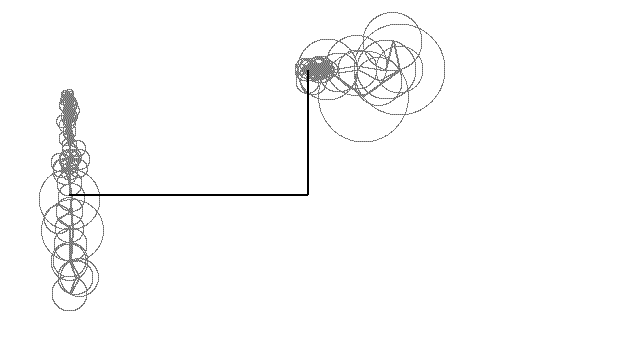
おまけ

こういうこともできます。

円運動の重ね合わせでお絵かき【フーリエ変換】

作品例

目次

大まかな流れ

環境

手順

PowerPointで絵を描く

.pptxを.zipに書き換えて解凍する

ベジェ曲線の実装

xmlから制御点を抽出して、曲線を描く

離散フーリエ変換

高速フーリエ変換

Pillowで絵を描く

完成

おまけ