2016年に作った資料を公開します。もう既にいろいろ古くなってる可能性が高いです。
Jupyter Notebook (IPython Notebook) とは
-
Python という名のプログラミング言語が使えるプログラミング環境。計算コードと計算結果を同じ場所に時系列で保存できるので、実験系における実験ノートのように、いつどんな処理を行って何を得たのか記録して再現するのに便利。
-
本実習ではまず、下のプログラムを順次実行してもらいます。各自の画面中の IPython Notebook のセルに順次入力して(コピペ可)、「Shift + Enter」してください。
-
最後に、課題を解いてもらいます。課題の結果を、指定する方法で指定するメールアドレスまで送信してください。
-
Python 2 と Python 3 で若干書き方が違う場合があるので注意してください。
# 図やグラフを図示するためのライブラリをインポートする。
import matplotlib.pyplot as plt
%matplotlib inline
# URL によるリソースへのアクセスを提供するライブラリをインポートする。
# import urllib # Python 2 の場合
import urllib.request # Python 3 の場合
簡単な折れ線グラフで時系列変化を図示する。
# ウェブ上のリソースを指定する
url = 'https://raw.githubusercontent.com/maskot1977/ipython_notebook/master/toydata/airmiles.txt'
# 指定したURLからリソースをダウンロードし、名前をつける。
# urllib.urlretrieve(url, 'airmiles.txt') # Python 2 の場合
urllib.request.urlretrieve(url, 'airmiles.txt') # Python 3 の場合
('airmiles.txt', <httplib.HTTPMessage instance at 0x10c6ba4d0>)
# ダウンロードしたファイルの冒頭だけ表示して中身を確認する
!head airmiles.txt
# ダウンロードしたファイルから、2つの列の数字をそれぞれリストに入れる。
x = []
y = []
for i, line in enumerate(open('airmiles.txt')):
    a = line.split()
    x.append(int(a[0]))
    y.append(int(a[1]))
# リストの中身を確認する。
print (x)
print (y)
[1937, 1938, 1939, 1940, 1941, 1942, 1943, 1944, 1945, 1946, 1947, 1948, 1949, 1950, 1951, 1952, 1953, 1954, 1955, 1956, 1957, 1958, 1959, 1960]
[412, 480, 683, 1052, 1385, 1418, 1634, 2178, 3362, 5948, 6109, 5981, 6753, 8003, 10566, 12528, 14760, 16769, 19819, 22362, 25340, 25343, 29269, 30514]
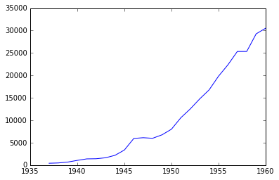
# とりあえず可視化してみる。
plt.plot(x,y)
[<matplotlib.lines.Line2D at 0x10eafb2d0>]
# もうちょっとカッコ良くする
plt.plot(x,y)
plt.title('Commercial Airline Mileage')
plt.xlabel('Year')
plt.ylabel('Passenger miles')
plt.show()
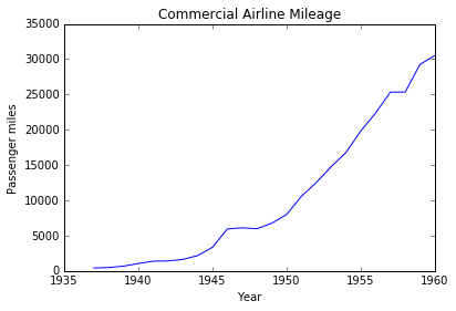
上図を「図1」と呼ぶことにします。課題1で、似たような図を作成してもらいます。
複数のデータの時系列を図示する
# ウェブ上のリソースを指定する
url = 'https://raw.githubusercontent.com/maskot1977/ipython_notebook/master/toydata/airquality.txt'
# 指定したURLからリソースをダウンロードし、名前をつける。
urllib.request.urlretrieve(url, 'airquality.txt')
('airquality.txt', <httplib.HTTPMessage instance at 0x10f036cf8>)
# ダウンロードしたファイルの冒頭だけ表示して中身を確認する
!head airquality.txt
# ダウンロードしたファイルから、それぞれの列の数字をリストに入れる。日付の情報は日付のオブジェクトに変換してリストに入れる。
import datetime
ozone = []
solar = []
wind = []
temp = []
date = []
for i, line in enumerate(open('airquality.txt')):
    if i == 0:
        continue
    else:
        a = line.split()
        if 'NA' in a:
            continue
        ozone.append(int(a[1]))
        solar.append(int(a[2]))
        wind.append(float(a[3]))
        temp.append(int(a[4]))
        month = int(a[5])
        day = int(a[6])
        date.append(datetime.datetime(1973, month, day))
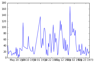
# まずは一種類のデータだけ図示してみる。
plt.plot(date, ozone)
[<matplotlib.lines.Line2D at 0x10f0ee690>]
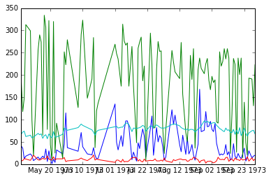
# すべてのデータを図示してみる。
plt.plot(date, ozone)
plt.plot(date, solar)
plt.plot(date, wind)
plt.plot(date, temp)
plt.show()
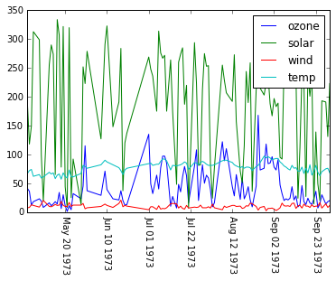
# もうちょっとカッコよくしてみる。
plt.plot(date, ozone, label='ozone')
plt.plot(date, solar, label='solar')
plt.plot(date, wind, label='wind')
plt.plot(date, temp, label='temp')
plt.legend()
plt.xticks(rotation=270)
plt.show()
# さらに見やすくしてみる
plt.figure(figsize=(8, 8))

plt.subplot(4, 1, 1)
plt.plot(date, ozone)
plt.title('airquality')
plt.xticks([])
plt.ylabel('Ozone')

plt.subplot(4, 1, 2)
plt.plot(date, solar)
plt.xticks([])
plt.ylabel('Solar')

plt.subplot(4, 1, 3)
plt.plot(date, wind)
plt.xticks([])
plt.ylabel('Wind')

plt.subplot(4, 1, 4)
plt.plot(date, temp)
plt.xticks(rotation=90)
plt.ylabel('Temp')
<matplotlib.text.Text at 0x10fb123d0>
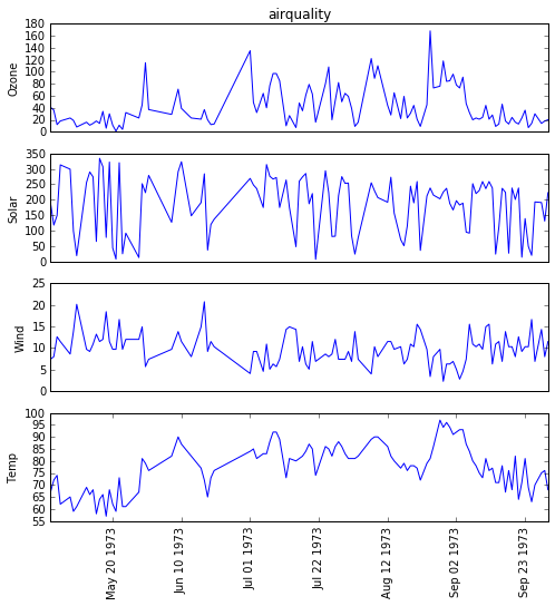
上図を「図2」と呼ぶことにします。課題2で、似たような図を作成してもらいます。
箱ひげ図(ボックスプロット)とバイオリンプロットを作成する
- 「箱ひげ図」(ボックスプロット)とは何か?知らない人は右記参照→ http://excelshogikan.com/qc/qc03/boxplot.html
# ウェブ上のリソースを指定する
url = 'https://raw.githubusercontent.com/maskot1977/ipython_notebook/master/toydata/iris.txt'
# 指定したURLからリソースをダウンロードし、名前をつける。
urllib.urlretrieve(url, 'iris.txt')
('iris.txt', <httplib.HTTPMessage instance at 0x10f765d40>)
# ダウンロードしたファイルの冒頭だけ表示して中身を確認する
!head iris.txt
# ダウンロードしたファイルから、4つの列の数字をそれぞれ4つのリストに入れる。
x1 = []
x2 = []
x3 = []
x4 = []
for i, line in enumerate(open('iris.txt')):
    if i == 0:
        continue
    else:
        a = line.split("\t")
        x1.append(float(a[1]))
        x2.append(float(a[2]))
        x3.append(float(a[3]))
        x4.append(float(a[4]))
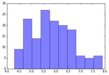
# x1のヒストグラム
plt.hist(x1, alpha=0.5)
(array([  9.,  23.,  14.,  27.,  22.,  20.,  18.,   6.,   5.,   6.]),
 array([ 4.3 ,  4.66,  5.02,  5.38,  5.74,  6.1 ,  6.46,  6.82,  7.18,
         7.54,  7.9 ]),
 <a list of 10 Patch objects>)
# もう少しカッコ良くする
plt.hist(x1, bins=20, alpha=0.5)
plt.title('Distribution of x1')
plt.xlabel('x1')
plt.ylabel('Occurence')
plt.show()
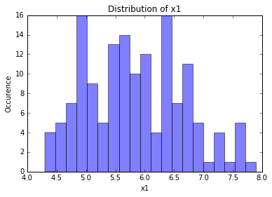
上記のヒストグラムを「図3」と呼ぶことにします。課題3で、似たような図を作成してもらいます。
# 箱ひげ図 (ボックスプロット)
fig = plt.figure()
ax = fig.add_subplot(111)
ax.boxplot([x1, x2, x3, x4])
ax.set_xticklabels(['x1', 'x2', 'x3', 'x4'], rotation=90)
plt.show()
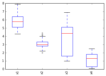
上記のボックスプロットを「図4」と呼ぶことにします。課題4で、似たような図を作成してもらいます。
# バイオリンプロット
fig = plt.figure()
ax = fig.add_subplot(111)
ax.violinplot([x1, x2, x3, x4])
ax.set_xticks([1, 2, 3, 4]) #データ範囲のどこに目盛りが入るかを指定する
ax.set_xticklabels(['x1', 'x2', 'x3', 'x4'], rotation=90)
plt.show()
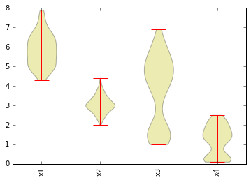
上記のバイオリンプロットを「図5」と呼ぶことにします。課題5で、似たような図を作成してもらいます。
ノード(点)のサイズや色に意味をもたせた散布図を作成する
# ウェブ上のリソースを指定する
url = 'https://raw.githubusercontent.com/maskot1977/ipython_notebook/master/toydata/USArrests.txt'
# 指定したURLからリソースをダウンロードし、名前をつける。
urllib.urlretrieve(url, 'USArrests.txt')
('USArrests.txt', <httplib.HTTPMessage instance at 0x10f19d488>)
!head USArrests.txt
# ダウンロードしたファイルから、2つの列の数字をそれぞれ4つのリストに入れる。
import datetime
state = []
murder = []
assault = []
urbanpop = []
rape = []
for i, line in enumerate(open('USArrests.txt')):
    if i == 0:
        continue
    else:
        a = line.split('\t')
        state.append(a[0])
        murder.append(float(a[1]))
        assault.append(int(a[2]))
        urbanpop.append(int(a[3]))
        rape.append(float(a[4]))
# ノード(点)のサイズや色に意味をもたせた散布図を作成する
names = state
x_axis = urbanpop
y_axis = murder
sizes = assault
colors = rape

name_label = "States"
x_label = "Urbanpop"
y_label = "Murder"
size_label = "Assault"
color_label = "Rape"

plt.figure(figsize=(20, 10))
for x, y, name in zip(x_axis, y_axis, names):
    plt.text(x, y, name, alpha=0.8, size=10)
plt.scatter(x_axis, y_axis, s=sizes, c=colors, alpha=0.8)
plt.colorbar(alpha=0.8)
plt.title("x=%s, y=%s, size=%s, color=%s" % (x_label, y_label, size_label, color_label))
plt.xlabel(x_label)
plt.ylabel(y_label)
plt.show()
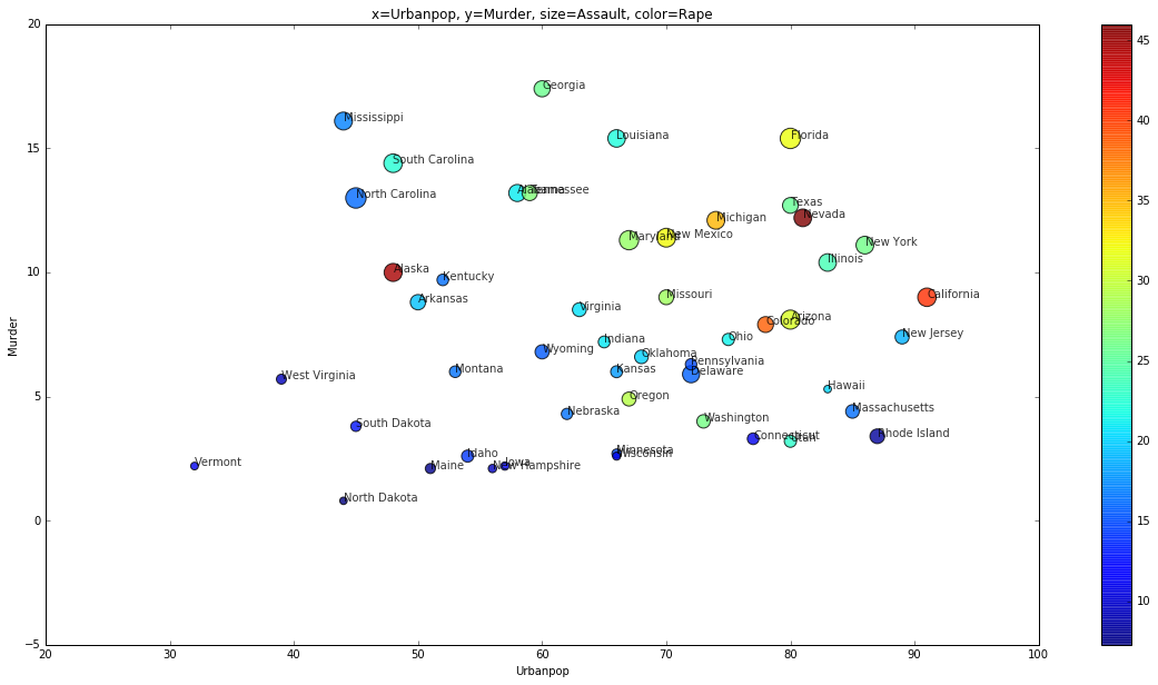
上図を「図6」と呼ぶことにします。課題6で、似たような図を作成してもらいます。
最後に、Scatter Matrix でデータの全体像を眺めてみましょう。
(本来は、最初にやるべきことですが、、、)
# 図やグラフを図示するためのライブラリをインポートする。
import matplotlib.pyplot as plt
%matplotlib inline
import pandas as pd # データフレームワーク処理のライブラリをインポート
from pandas.tools import plotting # 高度なプロットを行うツールのインポート
df = pd.read_csv('airquality.txt', sep='\t', na_values=".") # データの読み込み
pd.DataFrame(df).head() # 先頭N行を表示する。カラムのタイトルも確認する。
| Unnamed: 0 | Ozone | Solar.R | Wind | Temp | Month | Day | |
|---|---|---|---|---|---|---|---|
| 0 | 1 | 41 | 190 | 7.4 | 67 | 5 | 1 |
| 1 | 2 | 36 | 118 | 8.0 | 72 | 5 | 2 |
| 2 | 3 | 12 | 149 | 12.6 | 74 | 5 | 3 |
| 3 | 4 | 18 | 313 | 11.5 | 62 | 5 | 4 |
| 4 | 5 | NaN | NaN | 14.3 | 56 | 5 | 5 |
# 下記の関数にカラム名を入力すれば、Scatter Matrix が表示されます。
plotting.scatter_matrix(df[['Ozone', 'Solar.R', 'Wind', 'Temp']], figsize=(10, 10))
plt.show()
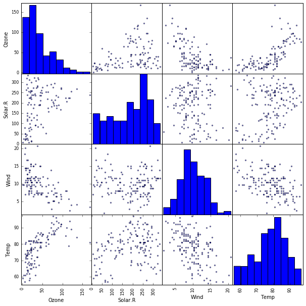
上図を「図7」と呼ぶことにします。課題7で、似たような図を作成してもらいます。
課題
新しいノートを開いて、以下の課題を解いてください。
-
課題1:下記リンクのデータを用いて、図1のような折れ線グラフを描いてください。
https://raw.githubusercontent.com/maskot1977/ipython_notebook/master/toydata/discoveries.txt -
課題2:図2を描き変えて、OzoneとSolar、WindとTempの折れ線グラフの位置をそれぞれ入れ替えた図にしてください。
-
課題3: 下記リンクのデータを用いて、図3のようなヒストグラムを作成してください。
https://raw.githubusercontent.com/maskot1977/ipython_notebook/master/toydata/islands.txt -
課題4:下記リンクのデータを用いて、Murder, Assault, UrbanPop, Rape について図4のようなボックスプロットを作成してください。
https://raw.githubusercontent.com/maskot1977/ipython_notebook/master/toydata/USArrests.txt -
課題5:下記リンクのデータを用いて、Murder, Assault, UrbanPop, Rape について図5のようなバイオリンプロットを作成してください。
https://raw.githubusercontent.com/maskot1977/ipython_notebook/master/toydata/USArrests.txt -
課題6:図6を描き変えて、横軸をMurder, 縦軸をAssault, サイズをUrbanPop, 色をRapeにした図にしてください。
-
課題7:下記リンクのデータを用いて、Murder, Assault, UrbanPop, Rape について図7のような Scatter Matrix を描いてください。
https://raw.githubusercontent.com/maskot1977/ipython_notebook/master/toydata/USArrests.txt
総合実験(Pythonプログラミング)4日間コース
本稿は「総合実験(Pythonプログラミング)4日間コース」シリーズ記事です。興味ある方は以下の記事も合わせてお読みください。