CNTK 2.2 Python API 解説 (6) - 画像分類タスクのための転移学習 (ResNet 18 モデル)

0. はじめに

◆ CNTK ( Microsoft Cognitive Toolkit ) 2.2 の Python API 解説第６弾です。
今回は、画像分類タスクのための転移学習を CNTK で遂行します。

ImageNet で訓練済みの既存のモデル (ResNet 18) があるとき、それを (類似した) 別の分野のデータセットに適合させるために、CNTK で転移学習 (= Transfer Learning) をどのように活用するかを示します。

転移学習は有用なテクニックです。例えば、新規の画像を異なるカテゴリーに分類する必要がありながら、しかし深層ニューラルネットワークをスクラッチからトレーニングするための十分なデータを持たない場合に利用可能なテクニックです。

本記事では、ImageNet 画像 (犬、猫、鳥 etc.) で訓練されたネットワークを花、そして動物 (羊/狼) のデータセットに適合させますが、転移学習は翻訳、音声合成、そして他の多くの分野のために既存のニューラルモデルを成功的に適合させてきました。

08093	08084	08081	08058

738519_d0394de9.jpg	Pair_of_Icelandic_Sheep.jpg	European_grey_wolf…	Wolf_je1-3.jpg

本記事の内容は :

1. 動作環境と Jupyter Notebook について
2. 転移学習
3. 準備 (インポートとデータ・ダウンロード)
4. 事前訓練されたモデル
5. 新しいデータセット
6. トレーニングと評価
7. 小さなデータセットの場合

本記事は以下の CNTK チュートリアルを参考にしています :

• CNTK 301: Image Recognition with Deep Transfer Learning

1. 動作環境と Jupyter Notebook について

動作環境

動作環境の構築が必要な場合には、Cognitive Toolkit 2.2 を Azure Linux GPU 仮想マシンにインストール を参考にしてください。Azure ポータルと Ubuntu Linux にある程度慣れていれば、30 分程度で以下のような環境が構築できるかと思います :

• Azure NC 仮想マシン with NVIDIA Tesla® K80 GPU
• Ubuntu 16.04 LTS
• NVIDIA CUDA 8.0 & cuDNN 6.0
• Anaconda 3 4.1.1
• CNTK 2.2 (for GPU)

Jupyter Notebook

また、本記事でも CNTK チュートリアルでも Jupyter Notebook を多用します。
Jupyter Notebook の利用方法については「CNTK 2.2 Python API 入門 (2)」の記事中の Jupyter Notebook の活用 を参照してください。

2. 転移学習

本記事は、訓練済みの既存のモデルがあるとき、それを類似した別の専門分野に適合させるために
CNTK で 転移学習 (= Transfer Learning) をどのように活用するかを示します。

問題設定

最初に、転移学習として扱う問題について説明します。
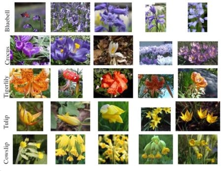
それぞれのカテゴリに分類される必要がある花の画像のセットが与えられたとします。下の画像はそのデータソースのサンプリングを示します :

しかしながら、Residual ネットワーク のような先端技術の分類器をトレーニングするためには、その画像の数が必要な量よりも圧倒的に少ないとします。

けれども、同時に、下で示されるような自然風景画像の注釈つきデータセットは豊富に持っているものとします (courtesy t-SNE visualization site) :

本記事では、データ不足問題に打ち勝つために複数のデータソースを利用する方法として深層転移学習を紹介します。

何故転移学習？

転移学習は有用なテクニックです。例えば、新規の画像を異なるカテゴリーに分類する必要がありながら
しかし深層ニューラルネットワーク (DNN) をスクラッチからトレーニングするための十分なデータを持たない場合に利用できます。

DNN をトレーニングするためには多くのデータを必要とし、総てがラベル付けされている必要がありますが、
現実にはしばしば手元にそのようなデータを持たないでしょう。
けれども、その問題となるネットワークが既に訓練済みのネットワークに類似している場合には、
転移学習を活用して、その訓練済みネットワークをラベル付けされたわずかの画像を持つ問題のために修正することができます。

転移学習とは何でしょう？

転移学習を用いて、既存のトレーニングされたモデルを流用してそれを新規の問題に適合させます。
本質的には、基本となるモデルのトレーニングの間に学習された特徴とコンセプト上に構築されます。

(今回のケースでは) 具体的には、畳み込み DNN (ResNet_18) を用いて ImageNet データから学習された特徴を使用して
最後の分類層を切り捨ててそれを新しい Dense 層で置き換えます。これは新しい分野のクラス・ラベルを予測します。

訓練された特徴を再利用してこの修正されたネットワークをトレーニングします。
新しい予測層の新しい重みだけか、ネットワーク全体の総ての重みをトレーニングするかは選択の余地があります。

転移学習は、例えば、既存の訓練されたモデルに類似した分野で画像の小さいセットだけを持つときに有用です。
深層ニューラルネットワークをスクラッチからトレーニングするためには数万の画像を必要としますが、
適合させようとしている特定の分野の特徴を既に学習したモデルを基にしてトレーニングすれば遥かに少ない画像ですみます。

今回の場合は、これは ImageNet 画像 (犬、猫、鳥 etc.) で訓練されたネットワークを 花、あるいは動物 (羊/狼) データセットに適合させることを意味しますが、転移学習は翻訳、音声合成、そして他の多くの分野のために既存のニューラルモデルを成功的に適合させてきている 点に注意してください。

3. 準備 (インポートとデータ・ダウンロード)

インポート

Microsoft の Cognitive Toolkit の Python 形式 cntk は、I/O・層定義・モデル訓練そして訓練されたモデルに問い合わせるための多くの有用なサブモジュールを含みます。
転移学習のためにはこれらの多くと、他に幾つかのコモンライブラリもまた必要とします :

In_[1]==>

from __future__ import print_function
import glob
import os
import numpy as np
from PIL import Image
# Some of the flowers data is stored as .mat files
from scipy.io import loadmat
from shutil import copyfile
import sys
import tarfile
import time

# Loat the right urlretrieve based on python version
try: 
    from urllib.request import urlretrieve 
except ImportError: 
    from urllib import urlretrieve
    
import zipfile

# Useful for being able to dump images into the Notebook
import IPython.display as D

# Import CNTK and helpers
import cntk as C

そして例によって２つの実行モードがあります。
Fast モードのためには 5 エポックについてモデルをトレーニングします。この結果は低い精度ですが開発のためには十分です。
Slow モードでは 20 エポックの間トレーニングをしますが、より良い結果のためにはより多くのエポック数が必要です :

In_[2]==>

isFast = True

データ・ダウンロード

さて、データセットをダウンロードします。
本記事では２つのデータセットを使用します: 一つは多くの花の画像を含み、そして他方はわずかばかりの羊と狼の画像を含みます。詳細については後述しますが、ここで行なうことはそれらをダウンロードしてアンパックすることです。

※ このノートブックは GPU が有効なマシンを持つ場合にのみ動作します :

In_[3]==>

C.device.try_set_default_device(C.device.gpu(0))

データセットは Jupyter Notebook の実行ディレクトリ下の DataSets フォルダにダウンロードされます。
download_unless_exists 関数は幾度かダウンロードを試みて、失敗すれば例外を見るでしょう :

In_[4]==>

# By default, we store data in the Examples/Image directory under CNTK
# If you're running this _outside_ of CNTK, consider changing this
# data_root = os.path.join('..', 'Examples', 'Image')
# data_root = os.path.join('.', 'data', 'Image')
data_root = os.path.join('.')
    
datasets_path = os.path.join(data_root, 'DataSets')
output_path = os.path.join('.', 'temp', 'Output')

def ensure_exists(path):
    if not os.path.exists(path):
        os.makedirs(path)

def write_to_file(file_path, img_paths, img_labels):
    with open(file_path, 'w+') as f:
        for i in range(0, len(img_paths)):
            f.write('%s\t%s\n' % (os.path.abspath(img_paths[i]), img_labels[i]))

def download_unless_exists(url, filename, max_retries=3):
    '''Download the file unless it already exists, with retry. Throws if all retries fail.'''
    if os.path.exists(filename):
        print('Reusing locally cached: ', filename)
    else:
        print('Starting download of {} to {}'.format(url, filename))
        retry_cnt = 0
        while True:
            try:
                urlretrieve(url, filename)
                print('Download completed.')
                return
            except:
                retry_cnt += 1
                if retry_cnt == max_retries:
                    print('Exceeded maximum retry count, aborting.')
                    raise
                print('Failed to download, retrying.')
                time.sleep(np.random.randint(1,10))
        
def download_model(model_root = os.path.join(data_root, 'PretrainedModels')):
    ensure_exists(model_root)
    resnet18_model_uri = 'https://www.cntk.ai/Models/ResNet/ResNet_18.model'
    resnet18_model_local = os.path.join(model_root, 'ResNet_18.model')
    download_unless_exists(resnet18_model_uri, resnet18_model_local)
    return resnet18_model_local

def download_flowers_dataset(dataset_root = os.path.join(datasets_path, 'Flowers')):
    ensure_exists(dataset_root)
    flowers_uris = [
        'http://www.robots.ox.ac.uk/~vgg/data/flowers/102/102flowers.tgz',
        'http://www.robots.ox.ac.uk/~vgg/data/flowers/102/imagelabels.mat',
        'http://www.robots.ox.ac.uk/~vgg/data/flowers/102/setid.mat'
    ]
    flowers_files = [
        os.path.join(dataset_root, '102flowers.tgz'),
        os.path.join(dataset_root, 'imagelabels.mat'),
        os.path.join(dataset_root, 'setid.mat')
    ]
    for uri, file in zip(flowers_uris, flowers_files):
        download_unless_exists(uri, file)
    tar_dir = os.path.join(dataset_root, 'extracted')
    if not os.path.exists(tar_dir):
        print('Extracting {} to {}'.format(flowers_files[0], tar_dir))
        os.makedirs(tar_dir)
        tarfile.open(flowers_files[0]).extractall(path=tar_dir)
    else:
        print('{} already extracted to {}, using existing version'.format(flowers_files[0], tar_dir))

    flowers_data = {
        'data_folder': dataset_root,
        'training_map': os.path.join(dataset_root, '6k_img_map.txt'),
        'testing_map': os.path.join(dataset_root, '1k_img_map.txt'),
        'validation_map': os.path.join(dataset_root, 'val_map.txt')
    }
    
    if not os.path.exists(flowers_data['training_map']):
        print('Writing map files ...')
        # get image paths and 0-based image labels
        image_paths = np.array(sorted(glob.glob(os.path.join(tar_dir, 'jpg', '*.jpg'))))
        image_labels = loadmat(flowers_files[1])['labels'][0]
        image_labels -= 1

        # read set information from .mat file
        setid = loadmat(flowers_files[2])
        idx_train = setid['trnid'][0] - 1
        idx_test = setid['tstid'][0] - 1
        idx_val = setid['valid'][0] - 1

        # Confusingly the training set contains 1k images and the test set contains 6k images
        # We swap them, because we want to train on more data
        write_to_file(flowers_data['training_map'], image_paths[idx_train], image_labels[idx_train])
        write_to_file(flowers_data['testing_map'], image_paths[idx_test], image_labels[idx_test])
        write_to_file(flowers_data['validation_map'], image_paths[idx_val], image_labels[idx_val])
        print('Map files written, dataset download and unpack completed.')
    else:
        print('Using cached map files.')
        
    return flowers_data
    
def download_animals_dataset(dataset_root = os.path.join(datasets_path, 'Animals')):
    ensure_exists(dataset_root)
    animals_uri = 'https://www.cntk.ai/DataSets/Animals/Animals.zip'
    animals_file = os.path.join(dataset_root, 'Animals.zip')
    download_unless_exists(animals_uri, animals_file)
    if not os.path.exists(os.path.join(dataset_root, 'Test')):
        with zipfile.ZipFile(animals_file) as animals_zip:
            print('Extracting {} to {}'.format(animals_file, dataset_root))
            animals_zip.extractall(path=os.path.join(dataset_root, '..'))
            print('Extraction completed.')
    else:
        print('Reusing previously extracted Animals data.')
        
    return {
        'training_folder': os.path.join(dataset_root, 'Train'),
        'testing_folder': os.path.join(dataset_root, 'Test')
    }

print('Downloading flowers and animals data-set, this might take a while...')
flowers_data = download_flowers_dataset()
animals_data = download_animals_dataset()
print('All data now available to the notebook!')

Downloading flowers and animals data-set, this might take a while...
Starting download of http://www.robots.ox.ac.uk/~vgg/data/flowers/102/102flowers.tgz to ./DataSets/Flowers/102flowers.tgz
Download completed.
Starting download of http://www.robots.ox.ac.uk/~vgg/data/flowers/102/imagelabels.mat to ./DataSets/Flowers/imagelabels.mat
Download completed.
Starting download of http://www.robots.ox.ac.uk/~vgg/data/flowers/102/setid.mat to ./DataSets/Flowers/setid.mat
Download completed.
Extracting ./DataSets/Flowers/102flowers.tgz to ./DataSets/Flowers/extracted
Writing map files ...
Map files written, dataset download and unpack completed.
Starting download of https://www.cntk.ai/DataSets/Animals/Animals.zip to ./DataSets/Animals/Animals.zip
Download completed.
Extracting ./DataSets/Animals/Animals.zip to ./DataSets/Animals
Extraction completed.
All data now available to the notebook!

ダウンロード完了後の DataSets 下のサブフォルダです :

$ ls -Fl DataSets/
total 8
drwxrwxr-x 4 masao masao 4096 Nov 21 18:15 Animals/
drwxrwxr-x 3 masao masao 4096 Nov 21 18:15 Flowers/

$ ls -Flh DataSets/Flowers/
total 330M
-rw-rw-r-- 1 masao masao 329M Nov 21 18:15 102flowers.tgz
-rw-rw-r-- 1 masao masao 481K Nov 21 18:15 1k_img_map.txt
-rw-rw-r-- 1 masao masao  80K Nov 21 18:15 6k_img_map.txt
drwxrwxr-x 3 masao masao 4.0K Nov 21 18:15 extracted/
-rw-rw-r-- 1 masao masao  502 Nov 21 18:15 imagelabels.mat
-rw-rw-r-- 1 masao masao  15K Nov 21 18:15 setid.mat
-rw-rw-r-- 1 masao masao  80K Nov 21 18:15 val_map.txt

$ ls -Flh DataSets/Animals/
total 5.4M
-rw-rw-r-- 1 masao masao 5.4M Nov 21 18:15 Animals.zip
drwxrwxr-x 4 masao masao 4.0K Nov 21 18:15 Test/
drwxrwxr-x 4 masao masao 4.0K Nov 21 18:15 Train/

花の画像は extracted/jpg ディレクトリに展開されます :

$ ls -lh DataSets/Flowers/extracted/jpg/ | head
total 347M
-rwxr-xr-x 1 masao masao  48K Feb 19  2009 image_00001.jpg
-rwxr-xr-x 1 masao masao  56K Feb 19  2009 image_00002.jpg
-rwxr-xr-x 1 masao masao  57K Feb 19  2009 image_00003.jpg
-rwxr-xr-x 1 masao masao  56K Feb 19  2009 image_00004.jpg
-rwxr-xr-x 1 masao masao  52K Feb 19  2009 image_00005.jpg
-rwxr-xr-x 1 masao masao  44K Feb 19  2009 image_00006.jpg
-rwxr-xr-x 1 masao masao  51K Feb 19  2009 image_00007.jpg
-rwxr-xr-x 1 masao masao  52K Feb 19  2009 image_00008.jpg
-rwxr-xr-x 1 masao masao  72K Feb 19  2009 image_00009.jpg

$ ls -lh DataSets/Flowers/extracted/jpg/ | tail
-rwxr-xr-x 1 masao masao  41K Feb 19  2009 image_08180.jpg
-rwxr-xr-x 1 masao masao  49K Feb 19  2009 image_08181.jpg
-rw-r--r-- 1 masao masao  31K Feb 19  2009 image_08182.jpg
-rwxr-xr-x 1 masao masao  25K Feb 19  2009 image_08183.jpg
-rw-r--r-- 1 masao masao  22K Feb 19  2009 image_08184.jpg
-rw-r--r-- 1 masao masao  37K Feb 19  2009 image_08185.jpg
-rwxr-xr-x 1 masao masao  39K Feb 19  2009 image_08186.jpg
-rwxr-xr-x 1 masao masao  30K Feb 19  2009 image_08187.jpg
-rwxr-xr-x 1 masao masao  31K Feb 19  2009 image_08188.jpg
-rwxr-xr-x 1 masao masao  32K Feb 19  2009 image_08189.jpg

動物画像の訓練データセットは非常に少なく、以下で総てリスティングされています :

$ ls -lhF DataSets/Animals/Train/
total 8.0K
drwxrwxr-x 2 masao masao 4.0K Nov 21 18:15 Sheep/
drwxrwxr-x 2 masao masao 4.0K Nov 21 18:15 Wolf/

$ ls -lhF DataSets/Animals/Train/Sheep/
total 2.3M
-rw-rw-r-- 1 masao masao 126K Nov 21 18:15 738519_d0394de9.jpg
-rw-rw-r-- 1 masao masao 110K Nov 21 18:15 A_sheep_in_the_long_grass.jpg
-rw-rw-r-- 1 masao masao  96K Nov 21 18:15 Cotswold_Sheep.jpg
-rw-rw-r-- 1 masao masao 133K Nov 21 18:15 Flock_of_sheep.jpg
-rw-rw-r-- 1 masao masao 167K Nov 21 18:15 Hambledon_Hill_Sheep.jpg
-rw-rw-r-- 1 masao masao 175K Nov 21 18:15 Karayaka-Sheep-1.jpg
-rw-rw-r-- 1 masao masao 172K Nov 21 18:15 Lleyn_sheep.jpg
-rw-rw-r-- 1 masao masao 107K Nov 21 18:15 Lundy_sheep_(head_detail).jpg
-rw-rw-r-- 1 masao masao 131K Nov 21 18:15 Pair_of_Icelandic_Sheep.jpg
-rw-rw-r-- 1 masao masao 208K Nov 21 18:15 Porkeri_sheep.jpg
-rw-rw-r-- 1 masao masao 172K Nov 21 18:15 Sheep-cumbria.jpg
-rw-rw-r-- 1 masao masao 119K Nov 21 18:15 Sheep_looking_1.jpg
-rw-rw-r-- 1 masao masao 214K Nov 21 18:15 Sheep_(Ovis_aries)_(8124797886).jpg
-rw-rw-r-- 1 masao masao 180K Nov 21 18:15 Sheep_sculpture_B.jpg
-rw-rw-r-- 1 masao masao 196K Nov 21 18:15 Swaledale_Sheep,_Lake_District,_England_-_June_2009.jpg

$ ls -lhF DataSets/Animals/Train/Wolf/
total 2.0M
-rw-rw-r-- 1 masao masao 166K Nov 21 18:15 European_grey_wolf_in_Prague_zoo.jpg
-rw-rw-r-- 1 masao masao  38K Nov 21 18:15 gray_wolf.jpg
-rw-rw-r-- 1 masao masao 122K Nov 21 18:15 Gray_Wolf,_Omega_Park,_QC.jpg
-rw-rw-r-- 1 masao masao 130K Nov 21 18:15 Grey_Wolf_7.jpg
-rw-rw-r-- 1 masao masao 152K Nov 21 18:15 Grey_wolf_P1130270.jpg
-rw-rw-r-- 1 masao masao 182K Nov 21 18:15 Lunca-European-Wolf.jpg
-rw-rw-r-- 1 masao masao 140K Nov 21 18:15 Mexican_Wolf_001.jpg
-rw-rw-r-- 1 masao masao 124K Nov 21 18:15 Mexican_Wolf_065.jpg
-rw-rw-r-- 1 masao masao 107K Nov 21 18:15 Mexican_Wolf_2_yfb-edit_1.jpg
-rw-rw-r-- 1 masao masao 122K Nov 21 18:15 Mexican_wolf_lounging.jpg
-rw-rw-r-- 1 masao masao 158K Nov 21 18:15 Scandinavian_grey_wolf_Canis_lupus.jpg
-rw-rw-r-- 1 masao masao 151K Nov 21 18:15 Wolf_dierenrijk_2009.jpg
-rw-rw-r-- 1 masao masao 110K Nov 21 18:15 wolf-eyes.jpg
-rw-rw-r-- 1 masao masao 150K Nov 21 18:15 Wolf_je1-3.jpg
-rw-rw-r-- 1 masao masao  91K Nov 21 18:15 Yellowstone-wolf-17120.jpg

4. 事前訓練されたモデル

事前訓練されたモデル (ResNet)

このタスクのための訓練されたモデルとして ResNet_18 を選択しました。
このモデルは Residual Network テクニックを使用して構築された、畳み込みニューラルネットワークです。
これを基本モデルとして転移学習により花と動物の分類のために適応させます。

Residual 深層学習は Microsoft Research 発のテクニックです。
入力データのメイン信号を "通過させる (passing through)" ことで、その結果としての層間で異なる残差部分上でネットワークは "学習" を遂行します :

このテクニックは、巨大なネットワーク上で勾配降下を悩ます問題を回避し、実際に遥かにより深いネットワークのトレーニングを可能にすることを証明しました。
より深い ResNet アーキテクチャの幾つか (50, 101 と 152-層) の可視化のためには、Kaiming He's GitHub を参照してください。

それではモデルをダウンロードします :

In_[5]==>

print('Downloading pre-trained model. Note: this might take a while...')
base_model_file = download_model()
print('Downloading pre-trained model complete!')

Downloading pre-trained model. Note: this might take a while...
Starting download of https://www.cntk.ai/Models/ResNet/ResNet_18.model to ./PretrainedModels/ResNet_18.model
Download completed.
Downloading pre-trained model complete!

$ ls PretrainedModels/ -lh
total 63M
-rw-rw-r-- 1 masao masao 63M Nov 21 18:24 ResNet_18.model

事前訓練されたモデルを探求する

どのようにモデルに問い合わせ可能かを示すために ResNet_18 の層の総てを出力表示してみます。
ResNet_18 と異なるモデルを使用するためには、使用するための適切な最後の隠れ層と特徴層を発見する必要があるだけです。
CNTK は、モデル詳細の総てをダンプするための cntk.loging.graph の下の便利な get_node_outputs メソッドを提供しています :

In_[6]==>

# モデルの位置と特徴を定義します。
base_model = {
    'model_file': base_model_file,
    'feature_node_name': 'features',
    'last_hidden_node_name': 'z.x',
    # チャネル x 高さ x 幅
    'image_dims': (3, 224, 224)
}

# モデルの総ての層を出力表示します。
print('Loading {} and printing all layers:'.format(base_model['model_file']))
node_outputs = C.logging.get_node_outputs(C.load_model(base_model['model_file']))
for l in node_outputs: print("  {0} {1}".format(l.name, l.shape))

Loading ./PretrainedModels/ResNet_18.model and printing all layers:
  ce ()
  errs ()
  top5Errs ()
  z (1000,)
  ce ()
  z (1000,)
  z.PlusArgs[0] (1000,)
  z.x (512, 1, 1)
  z.x.x.r (512, 7, 7)
  z.x.x.p (512, 7, 7)
  z.x.x.b (512, 7, 7)
  z.x.x.b.x.c (512, 7, 7)
  z.x.x.b.x (512, 7, 7)
  z.x.x.b.x._ (512, 7, 7)
  z.x.x.b.x._.x.c (512, 7, 7)
  z.x.x.x.r (512, 7, 7)
  z.x.x.x.p (512, 7, 7)
  z.x.x.x.b (512, 7, 7)
  z.x.x.x.b.x.c (512, 7, 7)
  z.x.x.x.b.x (512, 7, 7)
  z.x.x.x.b.x._ (512, 7, 7)
  z.x.x.x.b.x._.x.c (512, 7, 7)
  _z.x.x.x.r (512, 7, 7)
  _z.x.x.x.p (512, 7, 7)
  _z.x.x.x.b (512, 7, 7)
  _z.x.x.x.b.x.c (512, 7, 7)
  _z.x.x.x.b.x (512, 7, 7)
  _z.x.x.x.b.x._ (512, 7, 7)
  _z.x.x.x.b.x._.x.c (512, 7, 7)
  z.x.x.x.x.r (256, 14, 14)
  z.x.x.x.x.p (256, 14, 14)
  z.x.x.x.x.b (256, 14, 14)
  z.x.x.x.x.b.x.c (256, 14, 14)
  z.x.x.x.x.b.x (256, 14, 14)
  z.x.x.x.x.b.x._ (256, 14, 14)
  z.x.x.x.x.b.x._.x.c (256, 14, 14)
  z.x.x.x.x.x.r (256, 14, 14)
  z.x.x.x.x.x.p (256, 14, 14)
  z.x.x.x.x.x.b (256, 14, 14)
  z.x.x.x.x.x.b.x.c (256, 14, 14)
  z.x.x.x.x.x.b.x (256, 14, 14)
  z.x.x.x.x.x.b.x._ (256, 14, 14)
  z.x.x.x.x.x.b.x._.x.c (256, 14, 14)
  z.x.x.x.x.x.x.r (128, 28, 28)
  z.x.x.x.x.x.x.p (128, 28, 28)
  z.x.x.x.x.x.x.b (128, 28, 28)
  z.x.x.x.x.x.x.b.x.c (128, 28, 28)
  z.x.x.x.x.x.x.b.x (128, 28, 28)
  z.x.x.x.x.x.x.b.x._ (128, 28, 28)
  z.x.x.x.x.x.x.b.x._.x.c (128, 28, 28)
  z.x.x.x.x.x.x.x.r (128, 28, 28)
  z.x.x.x.x.x.x.x.p (128, 28, 28)
  z.x.x.x.x.x.x.x.b (128, 28, 28)
  z.x.x.x.x.x.x.x.b.x.c (128, 28, 28)
  z.x.x.x.x.x.x.x.b.x (128, 28, 28)
  z.x.x.x.x.x.x.x.b.x._ (128, 28, 28)
  z.x.x.x.x.x.x.x.b.x._.x.c (128, 28, 28)
  z.x.x.x.x.x.x.x.x.r (64, 56, 56)
  z.x.x.x.x.x.x.x.x.p (64, 56, 56)
  z.x.x.x.x.x.x.x.x.b (64, 56, 56)
  z.x.x.x.x.x.x.x.x.b.x.c (64, 56, 56)
  z.x.x.x.x.x.x.x.x.b.x (64, 56, 56)
  z.x.x.x.x.x.x.x.x.b.x._ (64, 56, 56)
  z.x.x.x.x.x.x.x.x.b.x._.x.c (64, 56, 56)
  z.x.x.x.x.x.x.x.x.x.r (64, 56, 56)
  z.x.x.x.x.x.x.x.x.x.p (64, 56, 56)
  z.x.x.x.x.x.x.x.x.x.b (64, 56, 56)
  z.x.x.x.x.x.x.x.x.x.b.x.c (64, 56, 56)
  z.x.x.x.x.x.x.x.x.x.b.x (64, 56, 56)
  z.x.x.x.x.x.x.x.x.x.b.x._ (64, 56, 56)
  z.x.x.x.x.x.x.x.x.x.b.x._.x.c (64, 56, 56)
  z.x.x.x.x.x.x.x.x.x (64, 56, 56)
  z.x.x.x.x.x.x.x.x.x.x (64, 112, 112)
  z.x.x.x.x.x.x.x.x.x.x._ (64, 112, 112)
  z.x.x.x.x.x.x.x.x.x.x._.x.c (64, 112, 112)
  z.x.x.x.x.x.x.x.s (128, 28, 28)
  z.x.x.x.x.x.x.x.s.x.c (128, 28, 28)
  z.x.x.x.x.x.s (256, 14, 14)
  z.x.x.x.x.x.s.x.c (256, 14, 14)
  z.x.x.x.s (512, 7, 7)
  z.x.x.x.s.x.c (512, 7, 7)
  errs ()
  top5Errs ()

5. 新しいデータセット

花のデータセットは Oxford Visual Geometry Group 由来のもので、UK で一般的な花の 102 の異なるカテゴリーを含みます。それはおよそ 8000 画像を持ち、訓練、テストそして検証セット間で分割されます。
より詳細な情報は VGG homepage for the dataset を参照してください。

データの幾つかを見てみましょう :

In_[7]==>

def plot_images(images, subplot_shape):
    plt.style.use('ggplot')
    fig, axes = plt.subplots(*subplot_shape)
    for image, ax in zip(images, axes.flatten()):
        ax.imshow(image.reshape(28, 28), vmin = 0, vmax = 1.0, cmap = 'gray')
        ax.axis('off')
    plt.show()

In_[8]==>

flowers_image_dir = os.path.join(flowers_data['data_folder'], 'extracted', 'jpg')


for image in ['08093', '08084', '08081', '08058']:
    D.display(D.Image(os.path.join(flowers_image_dir, 'image_{}.jpg'.format(image)), width=100, height=100))

08093	08084	08081	08058

6. トレーニングと評価

6-1. 転移学習モデルをトレーニングする

下のコードブロックでは、事前訓練された ResNet_18 モデルをロードしてそれをクローンする一方で最後の features 層を引き剥がしています。モデルをクローンするのは、訓練された同じモデルを複数回再利用するため、i.e. 異なることのために訓練するためです。
従って、単一のタスクのためにトレーニングするだけならば厳密にはこれは必要ありませんが、
これは CloneMethod.share を使用しない理由で、新しいパラメータを学習することを望んでいます。

freeze_weights が true である場合には、クローンする総ての層の重みを凍結して最後の新しい特徴層上の重みを学習するだけです。find_by_name を使用して最後の隠れ層 (z.x) を見つけて、それとその前にあるもの総てをクローンして、そして分類のための新しい Dense 層を追加します :

In_[9]==>

import cntk.io.transforms as xforms
ensure_exists(output_path)
np.random.seed(123)

# トレーニングとテストのために minibatch ソースを作成します。
def create_mb_source(map_file, image_dims, num_classes, randomize=True):
    transforms = [xforms.scale(width=image_dims[2], height=image_dims[1], channels=image_dims[0], interpolations='linear')]
    return C.io.MinibatchSource(C.io.ImageDeserializer(map_file, C.io.StreamDefs(
            features=C.io.StreamDef(field='image', transforms=transforms),
            labels=C.io.StreamDef(field='label', shape=num_classes))),
            randomize=randomize)

# 転移学習のためにネットワークモデルを作成します。
def create_model(model_details, num_classes, input_features, new_prediction_node_name='prediction', freeze=False):
    # Load the pretrained classification net and find nodes
    base_model = C.load_model(model_details['model_file'])
    feature_node = C.logging.find_by_name(base_model, model_details['feature_node_name'])
    last_node = C.logging.find_by_name(base_model, model_details['last_hidden_node_name'])

    # 望む層を固定された重みでクローンします。
    cloned_layers = C.combine([last_node.owner]).clone(
        C.CloneMethod.freeze if freeze else C.CloneMethod.clone,
        {feature_node: C.placeholder(name='features')})

    # クラス予測のための新しい dense 層を追加します。
    feat_norm = input_features - C.Constant(114)
    cloned_out = cloned_layers(feat_norm)
    z = C.layers.Dense(num_classes, activation=None, name=new_prediction_node_name) (cloned_out)

    return z

転移学習でも、他の一般的な CNTK モデル・トレーニングのようにモデルをトレーニングします。
つまり、入力ソースをインスタンス化し (画像データから MinibatchSource)、損失関数を定義し、そして多くのエポックの間トレーニングします。多クラス分類器ネットワークをトレーニングしますので、最終層は交差エントロピー Softmax で、そしてエラー関数は分類エラーです。両者ともに cntk.ops のユティリティ関数で便利に提供されます。

事前訓練されたモデルをトレーニングするとき、既存の重みを新しい分野に合うように適応させますが、
重みは既に正解に近いので (特によりプリミティブな特徴を見つけるより浅い層について)、
良い性能を得るためには、典型的には少ないサンプルと少ないエポックだけが必要とされます :

In_[10]==>

# 転移学習モデルをトレーニングします。
def train_model(model_details, num_classes, train_map_file,
                learning_params, max_images=-1):
    num_epochs = learning_params['max_epochs']
    epoch_size = sum(1 for line in open(train_map_file))
    if max_images > 0:
        epoch_size = min(epoch_size, max_images)
    minibatch_size = learning_params['mb_size']
    
    # minibatch ソースと入力変数を作成します。
    minibatch_source = create_mb_source(train_map_file, model_details['image_dims'], num_classes)
    image_input = C.input_variable(model_details['image_dims'])
    label_input = C.input_variable(num_classes)

    # リーダー・ストリームからネットワーク入力へのマッピングを定義します。
    input_map = {
        image_input: minibatch_source['features'],
        label_input: minibatch_source['labels']
    }

    # 転移学習モデルと損失関数をインスタンス化します。
    tl_model = create_model(model_details, num_classes, image_input, freeze=learning_params['freeze_weights'])
    ce = C.cross_entropy_with_softmax(tl_model, label_input)
    pe = C.classification_error(tl_model, label_input)

    # trainer オブジェクトをインスタンス化します。
    lr_schedule = C.learning_rate_schedule(learning_params['lr_per_mb'], unit=C.UnitType.minibatch)
    mm_schedule = C.momentum_schedule(learning_params['momentum_per_mb'])
    learner = C.momentum_sgd(tl_model.parameters, lr_schedule, mm_schedule, 
                           l2_regularization_weight=learning_params['l2_reg_weight'])
    trainer = C.Trainer(tl_model, (ce, pe), learner)

    # 画像のミニバッチを取得してモデル訓練を遂行します。
    print("Training transfer learning model for {0} epochs (epoch_size = {1}).".format(num_epochs, epoch_size))
    C.logging.log_number_of_parameters(tl_model)
    progress_printer = C.logging.ProgressPrinter(tag='Training', num_epochs=num_epochs)
    for epoch in range(num_epochs):       # loop over epochs
        sample_count = 0
        while sample_count < epoch_size:  # loop over minibatches in the epoch
            data = minibatch_source.next_minibatch(min(minibatch_size, epoch_size - sample_count), input_map=input_map)
            trainer.train_minibatch(data)                                    # update model with it
            sample_count += trainer.previous_minibatch_sample_count          # count samples processed so far
            progress_printer.update_with_trainer(trainer, with_metric=True)  # log progress
            if sample_count % (100 * minibatch_size) == 0:
                print ("Processed {0} samples".format(sample_count))

        progress_printer.epoch_summary(with_metric=True)

    return tl_model

訓練されたモデルを画像上で評価するとき、その画像を期待されるフォーマットに直さなければなりません。
今回の場合、パスから画像をロードし、それをモデルにより期待されるサイズにリサイズし、カラーチャネル (RGB to BGR) をリバースし、そして高さ、幅、そしてカラーチャネルに沿って連続する配列に変換するために、Image を使用します。これは 224 x 224 x 3 平坦化された配列に相当します、その上でモデルは訓練されました。

評価を行なうモデルは Softmax と Error 層を追加していませんでしたので、モデルで画像を評価するためには、入力データを model.eval メソッドに送り、確率を生成するために結果に渡り softmax して、そして予測されたクラスを決定するために NumPy の argmax メソッドを使用します。

それから全体に渡るモデル精度を得るためにそれを真のラベルと比較します :

In_[11]==>

# 再訓練されたモデルを使用して単一の画像を評価します。
def eval_single_image(loaded_model, image_path, image_dims):
    # load and format image (resize, RGB -> BGR, CHW -> HWC)
    try:
        img = Image.open(image_path)
        
        if image_path.endswith("png"):
            temp = Image.new("RGB", img.size, (255, 255, 255))
            temp.paste(img, img)
            img = temp
        resized = img.resize((image_dims[2], image_dims[1]), Image.ANTIALIAS)
        bgr_image = np.asarray(resized, dtype=np.float32)[..., [2, 1, 0]]
        hwc_format = np.ascontiguousarray(np.rollaxis(bgr_image, 2))

        # モデル出力を計算します。
        arguments = {loaded_model.arguments[0]: [hwc_format]}
        output = loaded_model.eval(arguments)

        # softmax 確率を返します。
        sm = C.softmax(output[0])
        return sm.eval()
    except FileNotFoundError:
        print("Could not open (skipping file): ", image_path)
        return ['None']
        


# 提供されたモデルを使用して画像セットを評価します。
def eval_test_images(loaded_model, output_file, test_map_file, image_dims, max_images=-1, column_offset=0):
    num_images = sum(1 for line in open(test_map_file))
    if max_images > 0:
        num_images = min(num_images, max_images)
    if isFast:
        num_images = min(num_images, 300) #We will run through fewer images for test run
        
    print("Evaluating model output node '{0}' for {1} images.".format('prediction', num_images))

    pred_count = 0
    correct_count = 0
    np.seterr(over='raise')
    with open(output_file, 'wb') as results_file:
        with open(test_map_file, "r") as input_file:
            for line in input_file:
                tokens = line.rstrip().split('\t')
                img_file = tokens[0 + column_offset]
                probs = eval_single_image(loaded_model, img_file, image_dims)
                
                if probs[0]=='None':
                    print("Eval not possible: ", img_file)
                    continue

                pred_count += 1
                true_label = int(tokens[1 + column_offset])
                predicted_label = np.argmax(probs)
                if predicted_label == true_label:
                    correct_count += 1

                #np.savetxt(results_file, probs[np.newaxis], fmt="%.3f")
                if pred_count % 100 == 0:
                    print("Processed {0} samples ({1:.2%} correct)".format(pred_count, 
                                                                           (float(correct_count) / pred_count)))
                if pred_count >= num_images:
                    break
    print ("{0} of {1} prediction were correct".format(correct_count, pred_count))
    return correct_count, pred_count, (float(correct_count) / pred_count)

◆ 最終的に、これらのヘルパー関数を用いて、花のデータセット上でモデルをトレーニングして評価します。
下の learning_params を自由に調整して結果を観察してください。

※ モデルを既にトレーニングした場合に、新しいパラメータでモデルを再訓練することをノートブックに強制するためには force_retraining を True に設定できます。

In_[12]==>

force_retraining = True

max_training_epochs = 5 if isFast else 20

learning_params = {
    'max_epochs': max_training_epochs,
    'mb_size': 50,
    'lr_per_mb': [0.2]*10 + [0.1],
    'momentum_per_mb': 0.9,
    'l2_reg_weight': 0.0005,
    'freeze_weights': True
}

flowers_model = {
    'model_file': os.path.join(output_path, 'FlowersTransferLearning.model'),
    'results_file': os.path.join(output_path, 'FlowersPredictions.txt'),
    'num_classes': 102
}

# Train only if no model exists yet or if force_retraining is set to True
if os.path.exists(flowers_model['model_file']) and not force_retraining:
    print("Loading existing model from %s" % flowers_model['model_file'])
    trained_model = C.load_model(flowers_model['model_file'])
else:
    trained_model = train_model(base_model,
                                flowers_model['num_classes'], flowers_data['training_map'],
                                learning_params)
    trained_model.save(flowers_model['model_file'])
    print("Stored trained model at %s" % flowers_model['model_file'])

Fast_モード

Training transfer learning model for 5 epochs (epoch_size = 1020).
Training 52326 parameters in 2 parameter tensors.
Finished Epoch[1 of 5]: [Training] loss = 4.857732 * 1020, metric = 93.04% * 1020 25.533s ( 39.9 samples/s);
Finished Epoch[2 of 5]: [Training] loss = 1.729792 * 1020, metric = 39.80% * 1020 2.483s (410.7 samples/s);
Finished Epoch[3 of 5]: [Training] loss = 0.594812 * 1020, metric = 12.25% * 1020 2.497s (408.4 samples/s);
Finished Epoch[4 of 5]: [Training] loss = 0.263091 * 1020, metric = 2.84% * 1020 2.467s (413.4 samples/s);
Finished Epoch[5 of 5]: [Training] loss = 0.149180 * 1020, metric = 0.49% * 1020 2.472s (412.6 samples/s);
Stored trained model at ./temp/Output/FlowersTransferLearning.model

Slow_モード

Training transfer learning model for 20 epochs (epoch_size = 1020).
Training 52326 parameters in 2 parameter tensors.
Finished Epoch[1 of 20]: [Training] loss = 4.857732 * 1020, metric = 93.04% * 1020 39.530s ( 25.8 samples/s);
Finished Epoch[2 of 20]: [Training] loss = 1.729792 * 1020, metric = 39.80% * 1020 2.502s (407.6 samples/s);
Finished Epoch[3 of 20]: [Training] loss = 0.594812 * 1020, metric = 12.25% * 1020 2.511s (406.2 samples/s);
Finished Epoch[4 of 20]: [Training] loss = 0.263091 * 1020, metric = 2.84% * 1020 2.515s (405.6 samples/s);
Finished Epoch[5 of 20]: [Training] loss = 0.149180 * 1020, metric = 0.49% * 1020 2.534s (402.6 samples/s);
Finished Epoch[6 of 20]: [Training] loss = 0.108990 * 1020, metric = 0.10% * 1020 2.557s (398.9 samples/s);
Finished Epoch[7 of 20]: [Training] loss = 0.086560 * 1020, metric = 0.00% * 1020 2.541s (401.5 samples/s);
Finished Epoch[8 of 20]: [Training] loss = 0.066960 * 1020, metric = 0.10% * 1020 2.538s (401.8 samples/s);
Finished Epoch[9 of 20]: [Training] loss = 0.058221 * 1020, metric = 0.10% * 1020 2.526s (403.8 samples/s);
Finished Epoch[10 of 20]: [Training] loss = 0.051114 * 1020, metric = 0.00% * 1020 2.528s (403.5 samples/s);
Finished Epoch[11 of 20]: [Training] loss = 0.041367 * 1020, metric = 0.00% * 1020 2.537s (402.1 samples/s);
Finished Epoch[12 of 20]: [Training] loss = 0.039614 * 1020, metric = 0.00% * 1020 2.540s (401.6 samples/s);
Finished Epoch[13 of 20]: [Training] loss = 0.037401 * 1020, metric = 0.00% * 1020 2.536s (402.2 samples/s);
Finished Epoch[14 of 20]: [Training] loss = 0.039385 * 1020, metric = 0.00% * 1020 2.531s (403.1 samples/s);
Finished Epoch[15 of 20]: [Training] loss = 0.036598 * 1020, metric = 0.00% * 1020 2.554s (399.4 samples/s);
Finished Epoch[16 of 20]: [Training] loss = 0.036361 * 1020, metric = 0.00% * 1020 2.561s (398.3 samples/s);
Finished Epoch[17 of 20]: [Training] loss = 0.035010 * 1020, metric = 0.00% * 1020 2.549s (400.1 samples/s);
Finished Epoch[18 of 20]: [Training] loss = 0.032773 * 1020, metric = 0.00% * 1020 2.550s (400.0 samples/s);
Finished Epoch[19 of 20]: [Training] loss = 0.032610 * 1020, metric = 0.00% * 1020 2.547s (400.5 samples/s);
Finished Epoch[20 of 20]: [Training] loss = 0.030438 * 1020, metric = 0.00% * 1020 2.541s (401.3 samples/s);
Stored trained model at ./temp/Output/FlowersTransferLearning.model
CPU times: user 2min 34s, sys: 55.1 s, total: 3min 29s
Wall time: 1min 30s

※ Slow モードでもまだ損失は大きいので、精度を上げるためにはエポック数を増やす必要があります。

6-2 評価の実行

事前訓練された ResNet モデルから学習を転移させることにより新たに学習された花の分類器を評価します :

In_[13]==>

# Evaluate the test set
predict_correct, predict_total, predict_accuracy = \
   eval_test_images(trained_model, flowers_model['results_file'], flowers_data['testing_map'], base_model['image_dims'])
print("Done. Wrote output to %s" % flowers_model['results_file'])

Fast_モード

Evaluating model output node 'prediction' for 300 images.
Processed 100 samples (62.00% correct)
Processed 200 samples (65.00% correct)
Processed 300 samples (71.67% correct)
215 of 300 prediction were correct
Done. Wrote output to ./temp/Output/FlowersPredictions.txt

Slow_モード

Evaluating model output node 'prediction' for 6149 images.
Processed 100 samples (61.00% correct)
Processed 200 samples (63.00% correct)
Processed 300 samples (71.00% correct)
Processed 400 samples (68.50% correct)
Processed 500 samples (73.60% correct)
Processed 600 samples (75.17% correct)
Processed 700 samples (76.14% correct)
Processed 800 samples (75.25% correct)
Processed 900 samples (76.67% correct)
Processed 1000 samples (77.10% correct)
Processed 1100 samples (77.27% correct)
Processed 1200 samples (76.75% correct)
Processed 1300 samples (76.38% correct)
Processed 1400 samples (76.71% correct)
Processed 1500 samples (76.33% correct)
Processed 1600 samples (76.38% correct)
Processed 1700 samples (75.82% correct)
Processed 1800 samples (75.11% correct)
Processed 1900 samples (75.47% correct)
Processed 2000 samples (75.65% correct)
Processed 2100 samples (76.38% correct)
Processed 2200 samples (77.00% correct)
Processed 2300 samples (76.39% correct)
Processed 2400 samples (75.12% correct)
Processed 2500 samples (74.32% correct)
Processed 2600 samples (73.58% correct)
Processed 2700 samples (74.11% correct)
Processed 2800 samples (74.75% correct)
Processed 2900 samples (75.34% correct)
Processed 3000 samples (76.03% correct)
Processed 3100 samples (76.74% correct)
Processed 3200 samples (77.12% correct)
Processed 3300 samples (77.73% correct)
Processed 3400 samples (77.82% correct)
Processed 3500 samples (78.31% correct)
Processed 3600 samples (78.03% correct)
Processed 3700 samples (78.08% correct)
Processed 3800 samples (77.87% correct)
Processed 3900 samples (77.33% correct)
Processed 4000 samples (77.48% correct)
Processed 4100 samples (77.17% correct)
Processed 4200 samples (77.45% correct)
Processed 4300 samples (77.63% correct)
Processed 4400 samples (77.61% correct)
Processed 4500 samples (77.62% correct)
Processed 4600 samples (77.74% correct)
Processed 4700 samples (77.85% correct)
Processed 4800 samples (77.19% correct)
Processed 4900 samples (77.00% correct)
Processed 5000 samples (76.58% correct)
Processed 5100 samples (76.57% correct)
Processed 5200 samples (76.48% correct)
Processed 5300 samples (76.21% correct)
Processed 5400 samples (76.00% correct)
Processed 5500 samples (75.73% correct)
Processed 5600 samples (75.77% correct)
Processed 5700 samples (75.81% correct)
Processed 5800 samples (75.64% correct)
Processed 5900 samples (75.24% correct)
Processed 6000 samples (74.80% correct)
Processed 6100 samples (75.02% correct)
4616 of 6149 prediction were correct
Done. Wrote output to ./temp/Output/FlowersPredictions.txt

In_[14]==>

# Test: Accuracy on flower data
print ("Prediction accuracy: {0:.2%}".format(float(predict_correct) / predict_total))

Fast_モード

Prediction accuracy: 71.67%

Slow_モード

Prediction accuracy: 75.07%

※ 十分なトレーニングによって 94 % 前後まで精度が上がるとのことです。
100 エポックではせいぜい 80 % 程度の精度でしたので、少なくとも 1000 エポックはトレーニングを試す必要があるでしょう。

7. 小さなデータセットの場合

花のデータセットでは、数百の画像を持つ数百のクラスがありました。
クラスと画像のより小さなセットを持つ場合でも転移学習は依然として機能するでしょうか？

答えはイエスです、ダウンロードした動物のデータセットで簡単に検証してみましょう。
このデータセットは羊と狼のクラスのみと画像の非常に小さなセットから成ります (クラス毎に１ダースのオーダーです)。

まずは画像を 2,3 個見てみましょう :

In_[15]==>

sheep = ['738519_d0394de9.jpg', 'Pair_of_Icelandic_Sheep.jpg']
wolves = ['European_grey_wolf_in_Prague_zoo.jpg', 'Wolf_je1-3.jpg']
for image in [os.path.join('Sheep', f) for f in sheep] + [os.path.join('Wolf', f) for f in wolves]:
    D.display(D.Image(os.path.join(animals_data['training_folder'], image), width=100, height=100))

738519_d0394de9.jpg	Pair_of_Icelandic_Sheep.jpg	European_grey_wolf…	Wolf_je1-3.jpg

画像はクラス名を与えるネストされたフォルダ (i.e. Sheep と Wolf フォルダ) を持つ、Train と Test フォルダにストアされています :

In_[16]==>

# Set python version variable 
python_version = sys.version_info.major

def create_map_file_from_folder(root_folder, class_mapping, include_unknown=False, valid_extensions=['.jpg', '.jpeg', '.png']):
    map_file_name = os.path.join(root_folder, "map.txt")
    
    map_file = None

    if python_version == 3: 
        map_file = open(map_file_name , 'w', encoding='utf-8')
    else:
        map_file = open(map_file_name , 'w')

    for class_id in range(0, len(class_mapping)):
        folder = os.path.join(root_folder, class_mapping[class_id])
        if os.path.exists(folder):
            for entry in os.listdir(folder):
                filename = os.path.abspath(os.path.join(folder, entry))
                if os.path.isfile(filename) and os.path.splitext(filename)[1].lower() in valid_extensions:
                    try:
                        map_file.write("{0}\t{1}\n".format(filename, class_id))
                    except UnicodeEncodeError:
                        continue

    if include_unknown:
        for entry in os.listdir(root_folder):
            filename = os.path.abspath(os.path.join(root_folder, entry))
            if os.path.isfile(filename) and os.path.splitext(filename)[1].lower() in valid_extensions:
                try:
                    map_file.write("{0}\t-1\n".format(filename))
                except UnicodeEncodeError:
                    continue
                    
    map_file.close()  
    
    return map_file_name
  

def create_class_mapping_from_folder(root_folder):
    classes = []
    for _, directories, _ in os.walk(root_folder):
        for directory in directories:
            classes.append(directory)
    return np.asarray(classes)

animals_data['class_mapping'] = create_class_mapping_from_folder(animals_data['training_folder'])
animals_data['training_map'] = create_map_file_from_folder(animals_data['training_folder'], animals_data['class_mapping'])
# Since the test data includes some birds, set include_unknown
animals_data['testing_map'] = create_map_file_from_folder(animals_data['testing_folder'], animals_data['class_mapping'], 
                                                          include_unknown=True)

モデルのトレーニングを実行します :

In_[17]==>

animals_model = {
    'model_file': os.path.join(output_path, 'AnimalsTransferLearning.model'),
    'results_file': os.path.join(output_path, 'AnimalsPredictions.txt'),
    'num_classes': len(animals_data['class_mapping'])
}

if os.path.exists(animals_model['model_file']) and not force_retraining:
    print("Loading existing model from %s" % animals_model['model_file'])
    trained_model = C.load_model(animals_model['model_file'])
else:
    trained_model = train_model(base_model, 
                                animals_model['num_classes'], animals_data['training_map'],
                                learning_params)
    trained_model.save(animals_model['model_file'])
    print("Stored trained model at %s" % animals_model['model_file'])

Fast_モード

Training transfer learning model for 5 epochs (epoch_size = 30).
Training 1026 parameters in 2 parameter tensors.
Finished Epoch[1 of 5]: [Training] loss = 0.913316 * 30, metric = 46.67% * 30 0.627s ( 47.8 samples/s);
Finished Epoch[2 of 5]: [Training] loss = 0.643136 * 30, metric = 20.00% * 30 1.894s ( 15.8 samples/s);
Finished Epoch[3 of 5]: [Training] loss = 0.129176 * 30, metric = 3.33% * 30 0.066s (455.7 samples/s);
Finished Epoch[4 of 5]: [Training] loss = 0.056904 * 30, metric = 0.00% * 30 0.110s (273.0 samples/s);
Finished Epoch[5 of 5]: [Training] loss = 0.035230 * 30, metric = 0.00% * 30 0.099s (302.1 samples/s);
Stored trained model at ./temp/Output/AnimalsTransferLearning.model

Slow_モード

Training transfer learning model for 20 epochs (epoch_size = 30).
Training 1026 parameters in 2 parameter tensors.
Finished Epoch[1 of 20]: [Training] loss = 0.913316 * 30, metric = 46.67% * 30 0.944s ( 31.8 samples/s);
Finished Epoch[2 of 20]: [Training] loss = 0.643136 * 30, metric = 20.00% * 30 1.871s ( 16.0 samples/s);
Finished Epoch[3 of 20]: [Training] loss = 0.129176 * 30, metric = 3.33% * 30 0.066s (456.5 samples/s);
Finished Epoch[4 of 20]: [Training] loss = 0.056904 * 30, metric = 0.00% * 30 0.119s (251.6 samples/s);
Finished Epoch[5 of 20]: [Training] loss = 0.035230 * 30, metric = 0.00% * 30 0.091s (330.5 samples/s);
Finished Epoch[6 of 20]: [Training] loss = 0.015069 * 30, metric = 0.00% * 30 0.097s (308.5 samples/s);
Finished Epoch[7 of 20]: [Training] loss = 0.005843 * 30, metric = 0.00% * 30 0.094s (317.7 samples/s);
Finished Epoch[8 of 20]: [Training] loss = 0.002318 * 30, metric = 0.00% * 30 0.104s (288.8 samples/s);
Finished Epoch[9 of 20]: [Training] loss = 0.000982 * 30, metric = 0.00% * 30 0.110s (273.4 samples/s);
Finished Epoch[10 of 20]: [Training] loss = 0.000449 * 30, metric = 0.00% * 30 0.091s (329.2 samples/s);
Finished Epoch[11 of 20]: [Training] loss = 0.000222 * 30, metric = 0.00% * 30 0.097s (309.0 samples/s);
Finished Epoch[12 of 20]: [Training] loss = 0.000118 * 30, metric = 0.00% * 30 0.100s (300.7 samples/s);
Finished Epoch[13 of 20]: [Training] loss = 0.000067 * 30, metric = 0.00% * 30 0.100s (300.0 samples/s);
Finished Epoch[14 of 20]: [Training] loss = 0.000041 * 30, metric = 0.00% * 30 0.096s (311.9 samples/s);
Finished Epoch[15 of 20]: [Training] loss = 0.000026 * 30, metric = 0.00% * 30 0.104s (288.9 samples/s);
Finished Epoch[16 of 20]: [Training] loss = 0.000018 * 30, metric = 0.00% * 30 0.103s (291.6 samples/s);
Finished Epoch[17 of 20]: [Training] loss = 0.000012 * 30, metric = 0.00% * 30 0.093s (322.4 samples/s);
Finished Epoch[18 of 20]: [Training] loss = 0.000009 * 30, metric = 0.00% * 30 0.104s (288.3 samples/s);
Finished Epoch[19 of 20]: [Training] loss = 0.000007 * 30, metric = 0.00% * 30 0.095s (316.2 samples/s);
Finished Epoch[20 of 20]: [Training] loss = 0.000005 * 30, metric = 0.00% * 30 0.105s (285.4 samples/s);
Stored trained model at ./temp/Output/AnimalsTransferLearning.model

モデルが動物データのためにトレーニングされましたので、画像を評価してみましょう :

In_[18]==>

# evaluate test images
with open(animals_data['testing_map'], 'r') as input_file:
    for line in input_file:
        tokens = line.rstrip().split('\t')
        img_file = tokens[0]
        true_label = int(tokens[1])
        probs = eval_single_image(trained_model, img_file, base_model['image_dims'])

        if probs[0]=='None':
            continue
        class_probs = np.column_stack((probs, animals_data['class_mapping'])).tolist()
        class_probs.sort(key=lambda x: float(x[0]), reverse=True)
        predictions = ' '.join(['%s:%.3f' % (class_probs[i][1], float(class_probs[i][0])) \
                                for i in range(0, animals_model['num_classes'])])
        true_class_name = animals_data['class_mapping'][true_label] if true_label >= 0 else 'unknown'
        print('Class: %s, predictions: %s, image: %s' % (true_class_name, predictions, img_file))

Fast_モード

Class: Wolf, predictions: Wolf:0.989 Sheep:0.011, image: /home/ubuntu/ws.cntk/notebook3/DataSets/Animals/Test/Wolf/Kolmarden_Wolf.jpg
Class: Wolf, predictions: Sheep:0.719 Wolf:0.281, image: /home/ubuntu/ws.cntk/notebook3/DataSets/Animals/Test/Wolf/The_white_wolf_by_Lunchi.jpg
Class: Wolf, predictions: Wolf:0.926 Sheep:0.074, image: /home/ubuntu/ws.cntk/notebook3/DataSets/Animals/Test/Wolf/Iberian_Wolf.jpg
Class: Wolf, predictions: Wolf:0.994 Sheep:0.006, image: /home/ubuntu/ws.cntk/notebook3/DataSets/Animals/Test/Wolf/9-wolf-profile-full.jpg
Class: Wolf, predictions: Wolf:0.998 Sheep:0.002, image: /home/ubuntu/ws.cntk/notebook3/DataSets/Animals/Test/Wolf/Canis_lupus_occidentalis.jpg
Class: Sheep, predictions: Sheep:0.957 Wolf:0.043, image: /home/ubuntu/ws.cntk/notebook3/DataSets/Animals/Test/Sheep/Swaledale_sheep.jpg
Class: Sheep, predictions: Sheep:0.998 Wolf:0.002, image: /home/ubuntu/ws.cntk/notebook3/DataSets/Animals/Test/Sheep/Icelandic_sheep_summer_06.jpg
Class: Sheep, predictions: Sheep:1.000 Wolf:0.000, image: /home/ubuntu/ws.cntk/notebook3/DataSets/Animals/Test/Sheep/Icelandic_breed_sheep.jpg
Class: Sheep, predictions: Sheep:0.995 Wolf:0.005, image: /home/ubuntu/ws.cntk/notebook3/DataSets/Animals/Test/Sheep/Sheep,_Stodmarsh_6.jpg
Class: Sheep, predictions: Sheep:1.000 Wolf:0.000, image: /home/ubuntu/ws.cntk/notebook3/DataSets/Animals/Test/Sheep/Romney_sheep,_ewe_with_triplet_lambs_in_New_Zealand.jpg
Class: unknown, predictions: Sheep:0.944 Wolf:0.056, image: /home/ubuntu/ws.cntk/notebook3/DataSets/Animals/Test/Weaver_bird.jpg
Class: unknown, predictions: Sheep:0.887 Wolf:0.113, image: /home/ubuntu/ws.cntk/notebook3/DataSets/Animals/Test/quetzal-bird.jpg
Class: unknown, predictions: Wolf:0.970 Sheep:0.030, image: /home/ubuntu/ws.cntk/notebook3/DataSets/Animals/Test/Bird_in_flight_wings_spread.jpg

Slow_モード

Class: Wolf, predictions: Wolf:1.000 Sheep:0.000, image: /home/ubuntu/ws.cntk/notebook3/DataSets/Animals/Test/Wolf/Kolmarden_Wolf.jpg
Class: Wolf, predictions: Wolf:0.860 Sheep:0.140, image: /home/ubuntu/ws.cntk/notebook3/DataSets/Animals/Test/Wolf/The_white_wolf_by_Lunchi.jpg
Class: Wolf, predictions: Wolf:1.000 Sheep:0.000, image: /home/ubuntu/ws.cntk/notebook3/DataSets/Animals/Test/Wolf/Iberian_Wolf.jpg
Class: Wolf, predictions: Wolf:1.000 Sheep:0.000, image: /home/ubuntu/ws.cntk/notebook3/DataSets/Animals/Test/Wolf/9-wolf-profile-full.jpg
Class: Wolf, predictions: Wolf:1.000 Sheep:0.000, image: /home/ubuntu/ws.cntk/notebook3/DataSets/Animals/Test/Wolf/Canis_lupus_occidentalis.jpg
Class: Sheep, predictions: Sheep:0.999 Wolf:0.001, image: /home/ubuntu/ws.cntk/notebook3/DataSets/Animals/Test/Sheep/Swaledale_sheep.jpg
Class: Sheep, predictions: Sheep:1.000 Wolf:0.000, image: /home/ubuntu/ws.cntk/notebook3/DataSets/Animals/Test/Sheep/Icelandic_sheep_summer_06.jpg
Class: Sheep, predictions: Sheep:1.000 Wolf:0.000, image: /home/ubuntu/ws.cntk/notebook3/DataSets/Animals/Test/Sheep/Icelandic_breed_sheep.jpg
Class: Sheep, predictions: Sheep:1.000 Wolf:0.000, image: /home/ubuntu/ws.cntk/notebook3/DataSets/Animals/Test/Sheep/Sheep,_Stodmarsh_6.jpg
Class: Sheep, predictions: Sheep:1.000 Wolf:0.000, image: /home/ubuntu/ws.cntk/notebook3/DataSets/Animals/Test/Sheep/Romney_sheep,_ewe_with_triplet_lambs_in_New_Zealand.jpg
Class: unknown, predictions: Wolf:0.660 Sheep:0.340, image: /home/ubuntu/ws.cntk/notebook3/DataSets/Animals/Test/Weaver_bird.jpg
Class: unknown, predictions: Wolf:0.877 Sheep:0.123, image: /home/ubuntu/ws.cntk/notebook3/DataSets/Animals/Test/quetzal-bird.jpg
Class: unknown, predictions: Wolf:1.000 Sheep:0.000, image: /home/ubuntu/ws.cntk/notebook3/DataSets/Animals/Test/Bird_in_flight_wings_spread.jpg

※ テストセットには鳥の画像が混在していますが、これを除けば Fast モードでも良い精度を示しています。

以上