はじめに
最近Watson StudioのJupyter Notebookでアニメーションを表示できることを知ったので、その方法についてメモ書きします。
前提
- IBM Cloudでのアカウント登録
- Watson Studioのインスタンス作成
- Watson Studioのプロジェクト作成
までは済んでいることを前提とします。手順については、別途記事をアップしていますので、そちらを参照して下さい。
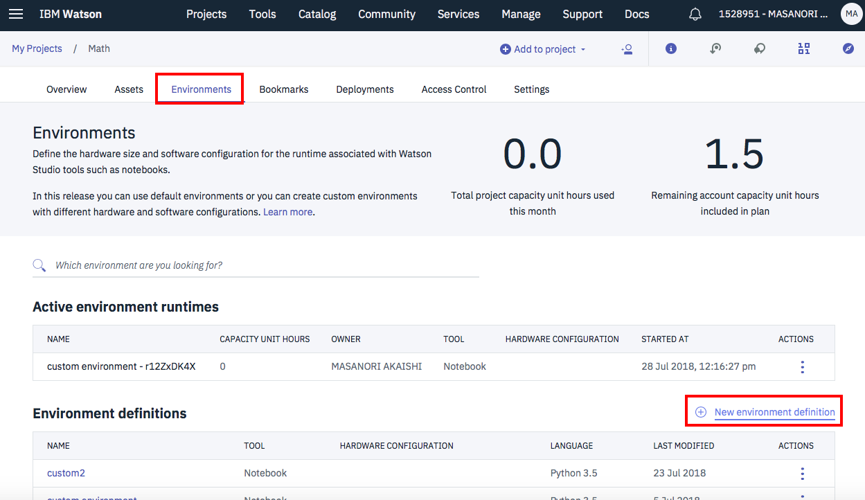
Environmentの設定
Watson StudioのJupyter Notebook環境でアニメーション表示をするためには、いくつかの不足モジュールの追加導入が必要です。
セルから !conda xxxや!pip xxxを実行すればいいのですが、Notebookがきたなくなるし、いちいち実行するのが面倒なので、アニメーション表示用Environmentを作成することにします。
プロジェクト管理の画面から「Environments」タブをクリックして、「New environment definition」をクリックします。
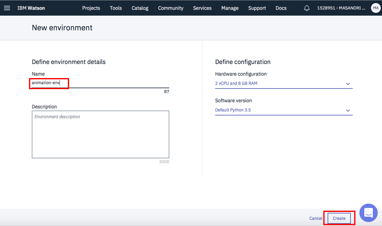
下の画面が出てきたら、名前を「animation-env」などとし、後はデフォルトで「Create」
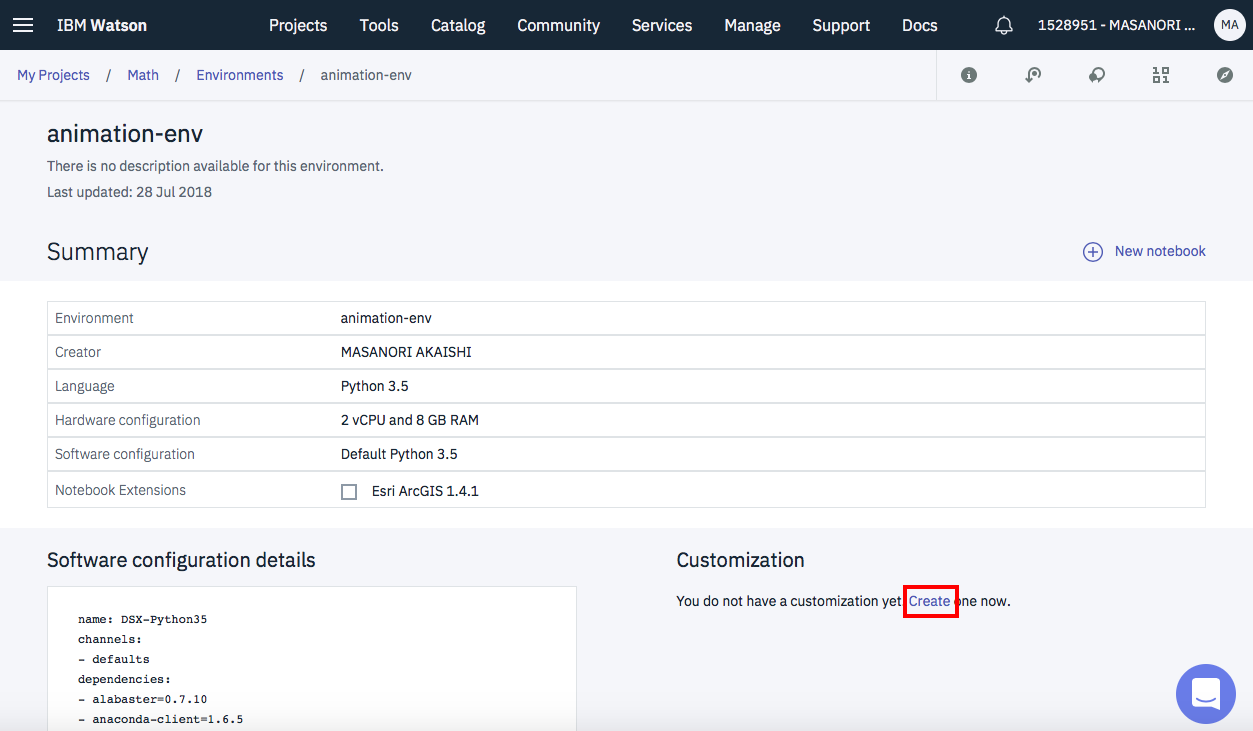
次の画面になったら、画面中程のCustomizationの欄にある「Create」リンクをクリック。
下の図のように「Customization」の欄ができるので、内容を下記のテキストに置き換えて「Apply」
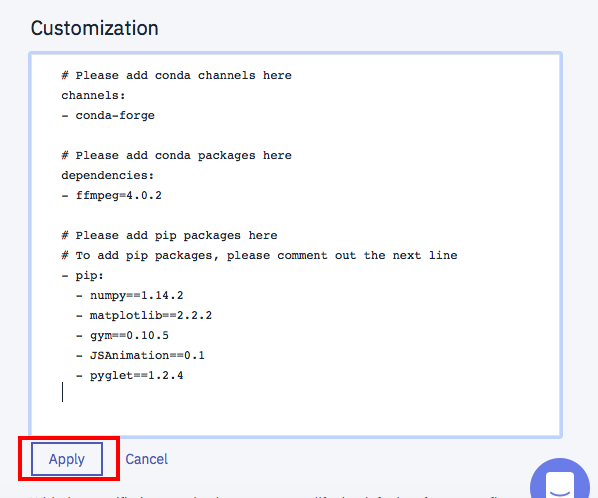
# Please add conda channels here
channels:
- conda-forge

# Please add conda packages here
dependencies:
- ffmpeg=4.0.2

# Please add pip packages here
# To add pip packages, please comment out the next line
- pip:
  - numpy==1.14.2
  - matplotlib==2.2.2
  - gym==0.10.5
  - JSAnimation==0.1
  - pyglet==1.2.4
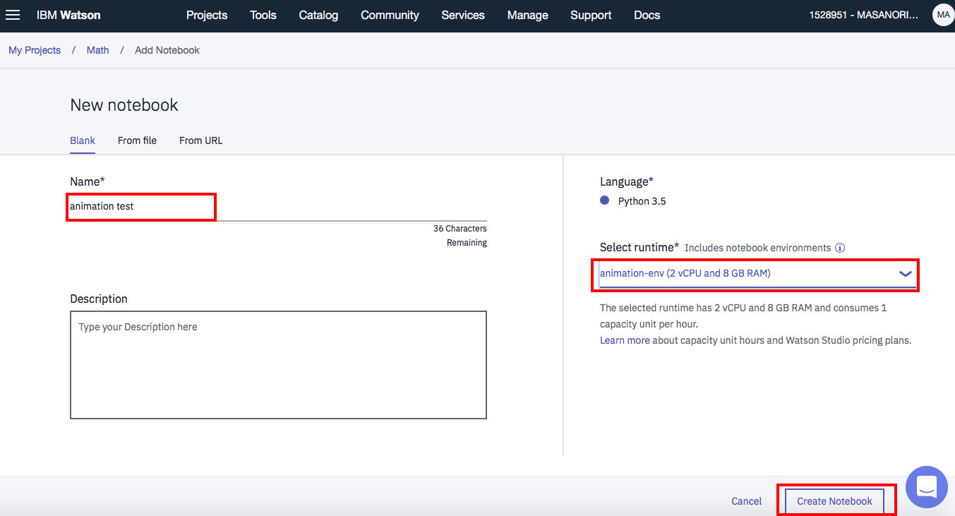
Notebookファイルの新規作成
保存が正常に終わったら、プロジェクト管理のメイン画面に戻ります。
「Add to project」から「Notebook」を選択し、新規ノートブック作成画面を表示します。
Notebook作成時、必ず「Select runtime」の欄で先ほど作ったEnvironmentである「animation-env」を選択するようにして下さい。
これは、既存Notebookファイルを読み込んでアニメーション表示する場合も同じです。
以下では、いくつかのサンプルコードを添付します。
サンプルコード1
正弦曲線による波動のアニメーションです。
初期設定
# 必要ライブラリのロード
%matplotlib inline
import numpy as np
import matplotlib.pyplot as plt
from matplotlib import animation, rc
from IPython.display import HTML

# 初期画面の描画
fig, ax = plt.subplots()

# x軸、y軸の範囲
ax.set_xlim(( 0, 2))
ax.set_ylim((-2, 2))

# グラフの線は枠だけ用意しておきます。
line, = ax.plot([], [], lw=2)
アニメーション表示
# 初期化関数
def init():
    line.set_data([], [])
    return (line,)

def animate(i):
    x = np.linspace(0, 2, 1000)
    y = np.sin(2 * np.pi * (x - 0.01 * i))
    line.set_data(x, y)
    return (line,)

# アニメーションの定義
anim = animation.FuncAnimation(fig, animate, init_func=init,
                               frames=100, interval=20, blit=True, repeat=True)

# アニメーションの描画
HTML(anim.to_html5_video())
うまくいくと、こんな画面が表示されます。

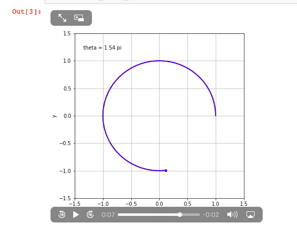
サンプルコード2
点が動いて円を描く様子です。
初期設定
# 必要なライブラリのロード
%matplotlib inline
from matplotlib import pyplot as plt
from matplotlib import animation
import numpy as np
from IPython.display import HTML

# 初期画面の表示
fig = plt.figure(figsize=(6,6))
ax = fig.add_subplot(111)
ax.set_ylim(-1.5, 1.5)
ax.set_xlim(-1.5, 1.5)
ax.set_xlabel('x')
ax.set_ylabel('y')
ax.grid()
time_text = ax.text(0.05, 0.9, '', transform=ax.transAxes)
アニメーション表示
# 円弧曲線と点の初期定義
curve, = ax.plot([], [], 'b-', lw=2)
point, = ax.plot([], [], 'bo', ms=4)
xx, yy = [], []

# 描画用パラメータ生成関数
def gen():
    for x in np.linspace(0,2,100):
        theta = x * np.pi
        yield np.cos(theta), np.sin(theta), x

# 描画用関数
def func(data):
    # パラメータの受け取り
    x, y, Rt = data
    # テキスト表示
    time_text.set_text('theta = %.2f pi' % Rt)
    # 円弧用ベクトルの生成
    xx.append(x)
    yy.append(y)
    # 円弧と点の描画
    curve.set_data(xx, yy)
    point.set_data(x, y)

# アニメーションの表示
anim = animation.FuncAnimation(fig,
        func, gen, blit=False, interval=100, repeat=False)
HTML(anim.to_html5_video())
うまくいくとこんな画面が表示されます。
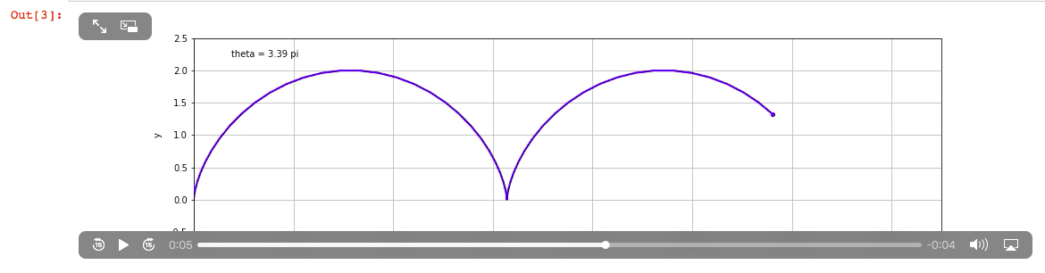
サンプルコード3
サイクロイド曲線です。
初期画面表示
# 必要ライブラリのロード
%matplotlib inline
from matplotlib import pyplot as plt
from matplotlib import animation
import numpy as np
from IPython.display import HTML

# 初期グラフの描画
fig = plt.figure(figsize=(15,4))
ax = fig.add_subplot(111)
ax.set_ylim(-0.5, 2.5)
ax.set_xlim(0, 15)
ax.set_xlabel('x')
ax.set_ylabel('y')
ax.grid()
time_text = ax.text(0.05, 0.9, '', transform=ax.transAxes)
アニメーションの表示
# 曲線と点の変数宣言
cycloid, = ax.plot([], [], 'b-', lw=2)
point, = ax.plot([], [], 'bo', ms=4)
xx, yy = [], []

# パラメータ生成関数
def gen():
    for theta in np.linspace(0,6*np.pi,100):
        yield theta-np.sin(theta), 1-np.cos(theta), theta

# アニメーション表示用関数
def func(data):
    # パラメータの受け取り
    x, y, Rt = data
    # テキスト表示
    time_text.set_text('theta = %.2f pi' % (Rt/np.pi))
    # 曲線のデータ生成
    xx.append(x)
    yy.append(y)
    # グラフ表示
    cycloid.set_data(xx, yy)
    point.set_data(x, y)

# アニメーション表示
anim = animation.FuncAnimation(fig,
        func, gen, blit=False, interval=100, repeat=False)
HTML(anim.to_html5_video())
うまくいくと、以下のようにサイクロイド曲線のアニメーションが表示されます。