はじめに
機械学習モデルの予測結果に対する解釈をいい感じに可視化してくれるライブラリとしてSHAPというものがあります。
SHAP (SHapley Additive exPlanations) is a game theoretic approach to explain the output of any machine learning model. It connects optimal credit allocation with local explanations using the classic Shapley values from game theory and their related extensions (see papers for details and citations).
(DeepLによる翻訳)
SHAP (SHapley Additive exPlanations)は、機械学習モデルの出力を説明するためのゲーム理論的アプローチである。これは、ゲーム理論の古典的なシャプリー値とその関連拡張を用いて、最適な信用配分を局所的な説明と結びつけます(詳細と引用は論文を参照)。
GithubのREADMEの冒頭の文章を引用
テーブルデータに対するSHAPの使い方は以下の記事がきれいにまとまっており参考になります。
公式のGithubのREADMEにも使い方が詳しく説明されています。
このSHAPはDeepLeaningのモデルにも使えるので、自然言語処理に対する適用方法を簡単にまとめてみます。
自然言語処理に対する適用方法は公式のチュートリアルを参考にしました。
今回はhuggingfaceのBERT(bert-base-cased)をファインチューニングしたモデルに対してSHAPを適用してみようと思います。
扱うデータセットは前回記事で紹介したhuggingfaceのdatasetsライブラリから取得できる感情分類用のemotionデータセットを使いたいと思います。
※SHAPの使い方(実装方法)に焦点を当てているため、SHAPの理論面には触れません。
詳しくは上記の参考記事や以下の元論文をご参照ください。
準備
ファインチューニングされた感情分類BERTモデルを用意するところまでざっと以下の通り実装します。
BERTの使い方については過去記事もご参照ください。
今回はGoogle colab上で動かすので、とりあえずGoogle Driveをcolabにマウントします。
# datasetsから取得したデータセットをtsv形式で一旦保存したいので、保存先としてGoogle Driveをするためにマウントしてます。
# colabにGoogle Driveをマウント
from google.colab import drive
drive.mount('/content/drive')
SHAPはpipでインストールできます。
# 必要なライブラリをpipでインストール
!pip install shap # SHAPはpipで簡単にインストールできます
!pip install datasets
!pip install transformers
必要な諸々のライブラリをインポートしておきます。
import shap
import datasets
from sklearn.metrics import classification_report
import pandas as pd
import numpy as np
import scipy as sp
import random
from IPython.display import display, HTML
import torch
import torch.nn as nn
import torch.nn.functional as F
import torch.optim as optim
import torchtext
from transformers import BertModel
from transformers import BertTokenizer

# データセット格納先
drive_dir = "drive/My Drive/Colab Notebooks/emotion_dataset/"
とりあえずBERTモデルは英語版の一番プレーン?なモデルを使います。
# cased->大文字と小文字を区別しない
# uncased->大文字と小文字を区別する
tokenizer = BertTokenizer.from_pretrained('bert-base-cased')
model = BertModel.from_pretrained("bert-base-cased")
huggingfaceのdatasetsライブラリから感情分析のデータセットemotionを使いたいのでdatasetsから取得します。
emotion_dataset = datasets.load_dataset('emotion')
torchtextでDataLoaderを作成するので、一旦データセットをtsvファイルに保存する
いちいちtsvファイルに保存しなくてもtorchtextで扱える方法があるのであれば、知らないだけです...
# まずはDataFrameに変換
# 学習データ
train_df = pd.DataFrame(emotion_dataset['train']['text'], columns=['text'])
train_df['label'] = emotion_dataset['train']['label']
# テストデータ
test_df = pd.DataFrame(emotion_dataset['test']['text'], columns=['text'])
test_df['label'] = emotion_dataset['test']['label']

# tsvファイルとして保存。保存先はマウントしたGoogle Drive
train_df.to_csv(drive_dir + 'train.tsv', sep='\t', index=False, header=None)
test_df.to_csv(drive_dir + 'test.tsv', sep='\t', index=False, header=None)

# 正解ラベルの数
# emotion datasetのラベルの数は6つです。
LABEL_NUM = len(set(train_df['label']))
# LABEL_NUM = 6

# ちなみに各ラベルの意味は以下の通りです。
labels = ["sadness", "joy", "love", "anger", "fear", "surprise"]

# 後ほど使うので、ラベルIDをラベルに変換、ラベルをラベルIDに変換する辞書をそれぞれ作成しておきます。
id2label = {i:labels[i] for i in range(len(labels))}
label2id = {label:labels.index(label) for label in labels}
torchtextを使ってDataLoaderを作成
# 英語版のBERTはtokenizerのoutputが辞書形式で返却されるようで
# 分かち書きのtoken idのリストは'input_ids'キーに格納されています。
# BERT modelの引数に対応した形のようです。
# Reference: https://huggingface.co/transformers/model_doc/bert.html
print(tokenizer(train_df['text'][0]))
# {'input_ids': [101, 178, 1238, 1204, 1631, 21820, 21896, 102], 'token_type_ids': [0, 0, 0, 0, 0, 0, 0, 0], 'attention_mask': [1, 1, 1, 1, 1, 1, 1, 1]}

def encode(text):
    return tokenizer(text)['input_ids']

TEXT = torchtext.data.Field(sequential=True, tokenize=encode, use_vocab=False, lower=False, include_lengths=True, batch_first=True, pad_token=0)
LABEL = torchtext.data.Field(sequential=False, use_vocab=False)

train_data, test_data = torchtext.data.TabularDataset.splits(path=drive_dir, train='train.tsv', test='test.tsv', format='tsv', fields=[('Text', TEXT), ('Label', LABEL)])

BATCH_SIZE = 32
train_iter, test_iter = torchtext.data.Iterator.splits((train_data, test_data), batch_sizes=(BATCH_SIZE, BATCH_SIZE), repeat=False, sort=False)
BERTによる感情分類モデルを定義します。
class BertClassifier(nn.Module):
  def __init__(self, base_model, label_num):
    super(BertClassifier, self).__init__()
    self.bert = base_model
    # BERTのアウトプットの次元数は768次元、label_numは正解ラベルの数を指定する
    self.linear = nn.Linear(768, label_num)

    # 重み初期化処理
    nn.init.normal_(self.linear.weight, std=0.02)
    nn.init.normal_(self.linear.bias, 0)

  def forward(self, encode_input):
    # Attentionの可視化も行いたいので、output_attentions=Trueを指定してます。
    output = self.bert(encode_input, output_attentions=True)

    # outputが辞書形式になっているので、必要な出力のキーを指定して取得する
    vec = output['last_hidden_state']
    attentions = output['attentions']

    # 先頭トークンCLSのベクトルだけ取得
    vec = vec[:,0,:]
    vec = vec.view(-1, 768)

    # 全結合層でクラス分類用に次元を変換
    vec = self.linear(vec)

    return F.log_softmax(vec, dim=1), attentions

classifier = BertClassifier(base_model=model, label_num=LABEL_NUM)
ファインチューニングの設定やら最適化関数、損失関数の定義をしておきます。
# まずは全パラメータを学習対象外にする
for param in classifier.parameters():
    param.requires_grad = False

# BERTモデルの最後の層を学習対象
for param in classifier.bert.encoder.layer[-1].parameters():
    param.requires_grad = True

# 最後の全結合層を学習対象
for param in classifier.linear.parameters():
    param.requires_grad = True

# 最適化関数、損失関数の定義
optimizer = optim.Adam([
    {'params': classifier.bert.encoder.layer[-1].parameters(), 'lr': 5e-5},
    {'params': classifier.linear.parameters(), 'lr': 1e-4}
])

loss_function = nn.NLLLoss()

device = torch.device("cuda:0" if torch.cuda.is_available() else "cpu")
classifier.to(device)
学習させます。とりあえず5エポックだけ回します。
for epoch in range(5):
  all_loss = 0
  for idx, batch in enumerate(train_iter):
    batch_loss = 0
    classifier.zero_grad()
    input_ids = batch.Text[0].to(device)
    label_ids = batch.Label.to(device)
    out, _ = classifier(input_ids)
    batch_loss = loss_function(out, label_ids)
    batch_loss.backward()
    optimizer.step()
    all_loss += batch_loss.item()
  print("epoch", epoch, "\t" , "loss", all_loss)
F1-scoreで精度を確認しておきます。
answer = []
prediction = []
with torch.no_grad():
    for batch in test_iter:

        text_tensor = batch.Text[0].to(device)
        label_tensor = batch.Label.to(device)

        score, _ = classifier(text_tensor)
        _, pred = torch.max(score, 1)

        prediction += list(pred.cpu().numpy())
        answer += list(label_tensor.cpu().numpy())
print(classification_report(prediction, answer, target_names=labels))
# surpriseは特にデータ数が少ないために他と比べてF1-scoreがやや小さめな結果となっているようです。
#              precision    recall  f1-score   support

#     sadness       0.92      0.91      0.91       589
#         joy       0.95      0.86      0.90       763
#        love       0.63      0.87      0.73       115
#       anger       0.81      0.94      0.87       237
#        fear       0.85      0.83      0.84       230
#    surprise       0.70      0.70      0.70        66

#    accuracy                           0.87      2000
#   macro avg       0.81      0.85      0.82      2000
# weighted avg       0.88      0.87      0.88      2000
SHAPを使ってモデルを解釈してみる
公式リファレンスのtext exampleを参考に実装します。
GithubのREADMEをみる限り、TensorFlowやKerasのモデルであればshap.DeepExplainerが使えるようですが(KerasのLSTMモデルの例)、huggingfaceのtransformersはshap.Explainerを使えばいいようですね。
以下では1文章に対する可視化方法と複数文章に対するSHAP値のサマリー情報の2つの可視化方法を紹介します。
shap.Explainerの使い方
引数がいくつかあり、それぞれの意味がよくわからなかったのですが、ソースコードにコメントで詳しい記載がされていたので、一部分を引用します。
class Explainer(Serializable):
    """ Uses Shapley values to explain any machine learning model or python function.

    This is the primary explainer interface for the SHAP library. It takes any combination
    of a model and masker and returns a callable subclass object that implements
    the particular estimation algorithm that was chosen.
    """

    def __init__(self, model, masker=None, link=links.identity, algorithm="auto", output_names=None, feature_names=None, **kwargs):
        """ Build a new explainer for the passed model.

        Parameters
        ----------
        model : object or function
            User supplied function or model object that takes a dataset of samples and
            computes the output of the model for those samples.

        masker : function, numpy.array, pandas.DataFrame, tokenizer, None, or a list of these for each model input
            The function used to "mask" out hidden features of the form `masked_args = masker(*model_args, mask=mask)`.
            It takes input in the same form as the model, but for just a single sample with a binary
            mask, then returns an iterable of masked samples. These
            masked samples will then be evaluated using the model function and the outputs averaged.
            As a shortcut for the standard masking using by SHAP you can pass a background data matrix
            instead of a function and that matrix will be used for masking. Domain specific masking
            functions are available in shap such as shap.ImageMasker for images and shap.TokenMasker
            for text. In addition to determining how to replace hidden features, the masker can also
            constrain the rules of the cooperative game used to explain the model. For example
            shap.TabularMasker(data, hclustering="correlation") will enforce a hierarchial clustering
            of coalitions for the game (in this special case the attributions are known as the Owen values).

        link : function
            The link function used to map between the output units of the model and the SHAP value units. By
            default it is shap.links.identity, but shap.links.logit can be useful so that expectations are
            computed in probability units while explanations remain in the (more naturally additive) log-odds
            units. For more details on how link functions work see any overview of link functions for generalized
            linear models.

        algorithm : "auto", "permutation", "partition", "tree", "kernel", "sampling", "linear", "deep", or "gradient"
            The algorithm used to estimate the Shapley values. There are many different algorithms that
            can be used to estimate the Shapley values (and the related value for constrained games), each
            of these algorithms have various tradeoffs and are preferrable in different situations. By
            default the "auto" options attempts to make the best choice given the passed model and masker,
            but this choice can always be overriden by passing the name of a specific algorithm. The type of
            algorithm used will determine what type of subclass object is returned by this constructor, and
            you can also build those subclasses directly if you prefer or need more fine grained control over
            their options.

        output_names : None or list of strings
            The names of the model outputs. For example if the model is an image classifier, then output_names would
            be the names of all the output classes. This parameter is optional. When output_names is None then
            the Explanation objects produced by this explainer will not have any output_names, which could effect
            downstream plots.
        """
まだいまいち理解しきれていないところがありますが、今回はmodel、masker、output_namesを指定して動かしています。
modelはちょっと注意が必要です。今回でいうと、分類モデルのインスタンスclassifierを指定しちゃいたくなりますが、こいつのインプットは自然文をid列に変換したテンソルです。id列に対してSHAP値を求めても、なんの単語や文章が出力に効いているかよくわからないので、modelには自然文をインプットできる形式で書き換えてあげる必要があります。
maskerにはトークナイザーを指定してやればよいようで、modelで指定したモデルと同じインプットで動くものを指定します。今回で言えばBERTモデルのトークナイザーのインスタンスtokenizer
をそのまま指定しています。
output_namesは正解ラベルで使っていたラベルの配列を指定します。
# shap.Explainerの引数modelに指定する関数を以下で定義
# 引数のsentencesは自然文の配列を想定しています。
# 自然文が1つだけの時はその文章を配列に変換してから使います。
# max_lengthはテストデータの最大長さを指定しています。
def f(sentences):
    input_ids = torch.tensor([tokenizer.encode(text, padding='max_length', max_length=68) for text in sentences]).to(device)
    with torch.no_grad():
        out, _ = classifier(input_ids)
    return out.detach().cpu()

# SHAP値を計算するインスタンスを生成する
explainer = shap.Explainer(model=f, masker=tokenizer, output_names=labels)

# あとはSHAP値を計算したい自然文の配列をexplainerに渡せばOK
# 後ほど実行するのでここではコメントアウトしますが、以下のように自然文をインプットすればOK
# shap_values = explainer(sentences)
Attentionとの比較も行いたいので諸々用意しておく
自然言語処理における説明性の可視化と言えばAttentionが思い浮かぶかと思います。
SHAPの可視化と同時に、どの単語がAttentionされているかも見比べてみようと思います。
# SHAP値を算出するときと同様の方法でAttentionの結果を得られる関数を用意しておく
def f_a(sentences):
    input_ids = torch.tensor([tokenizer.encode(text, padding='max_length', max_length=68) for text in sentences]).to(device)
    with torch.no_grad():
        _, attn = classifier(input_ids)
    return input_ids[0].detach().cpu(), attn[-1].detach().cpu()

# 以下2つの関数はAttentionの結果を単語にハイライトするためのものです。
# 以前書いた記事で使っていた関数を今回用に書き換えています。
def highlight(word, attn):
  html_color = '#%02X%02X%02X' % (255, int(255*(1 - attn)), int(255*(1 - attn)))
  return '<span style="background-color: {}">{}</span>'.format(html_color, word)

def mk_html(input_ids, attention_weight):
    # 文章の長さ分のzero tensorを宣言
    seq_len = attention_weight.size()[2]
    all_attens = torch.zeros(seq_len)

    # 12個のMulti Head Attentionの結果を全部足し合わせる
    # 最初の0はinput_idsは1文章だけを想定しているため
    # 次の0はCLSトークンのAttention結果を取得している、という意味です。
    for i in range(12):
        all_attens += attention_weight[0, i, 0, :]

    html = ""
    for word, attn in zip(input_ids, all_attens):
        if tokenizer.convert_ids_to_tokens([word.tolist()])[0] == "[SEP]":
            break
        html += highlight(tokenizer.convert_ids_to_tokens([word.numpy().tolist()])[0], attn) + " "

    return html
1つの文章に対して使ってみる
とりあえずランダムにテストデータから1文章引っ張ってきます。「i dont know if i should let go and feel that vain or should i wait and stay in vain」という文章がピックアップされて、正解、予測ともに「sadness」だそうです。
※DeepLによる翻訳「私は手放して、その虚しさを感じるべきか、それとも待って虚しさのままでいるべきかわからない。」
idx = random.randint(0,len(test_df))
sentence = test_df['text'][idx]
answer = id2label[test_df['label'][idx]]
predict = id2label[f([sentence]).argmax().item()]

# Attentionの計算
input_ids, attention = f_a([sentence])

print("元文章", sentence)
print("正解ラベル", answer)
print("予測ラベル", predict)
# 元文章 i dont know if i should let go and feel that vain or should i wait and stay in vain
# 正解ラベル sadness
# 予測ラベル sadness

# SHAP値を計算する
# sentenceは1文章だけなので、[]で囲って配列として渡してます。
shap_values = explainer([sentence])
shap.plots.textに計算されたSHAP値を以下のように渡します。
# Attention可視化
print("■Attentionの可視化結果")
html_output = mk_html(input_ids, attention)
display(HTML(html_output))
print()

print("■SHAPの可視化結果")
# shap.plots.textに計算したSHAP値を渡します。
# どの単語や句が予測ラベルにどれくらい(プラスの方向、マイナスの方向に)効いていたかを可視化します。
# 赤がプラス、青がマイナスの方向を表現しており、濃淡は度合いを表しています。
shap.plots.text(shap_values[0,:,predict])
どの単語や句が予測ラベルにどれくらい(プラスの方向、マイナスの方向に)効いていたかを可視化します。
赤がプラス、青がマイナスの方向を表現しており、濃淡は度合いを表しています。
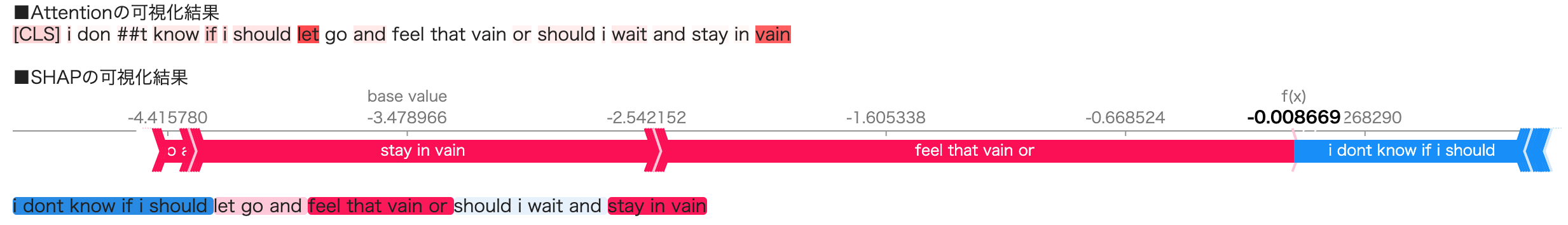
おそらく「vain(虚しい、はかない)」が一番sadnessっぽい単語だと思いますが、Attentionでは2つ目のvainに強くAttentionしているようで、SHAPでは「feel that vain or」や「stay in vain」がsadnessによく効いていたことがわかります。
Atteintionではどの単語が予測をする上で重要か(lossを下げてくれるか)、くらいしかわかりませんが、SHAPでは「i dont know if i should」が予測に対してマイナス方向に効いた、ということもわかります。(これが本当に妥当な結果かどうかはおいといて...)
以下のように、ラベルを指定しなければ、全ラベルに対して、各単語や句がどのラベルに効いていたかをHeat map形式でみることができます。
shap.plots.text(shap_values[0,:,])
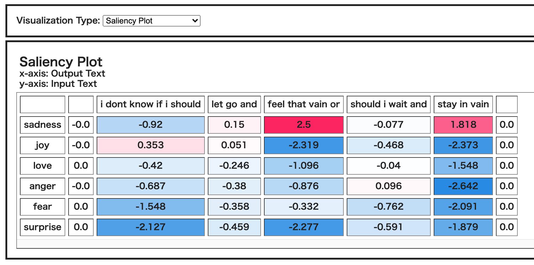
これを見ると、sadnessの方向に効いた「feel that vain or」「stay in vain」は例えばjoyに対してマイナス方向に効いていることがわかりますし、sadnessにマイナスの方向に効いていた「i dont know if i should」はjoyに対してプラス方向に効いているようです。sadnessの反対の意味に相当するjoyに対してこのような結果になったのは、なんだかしっくりきます。
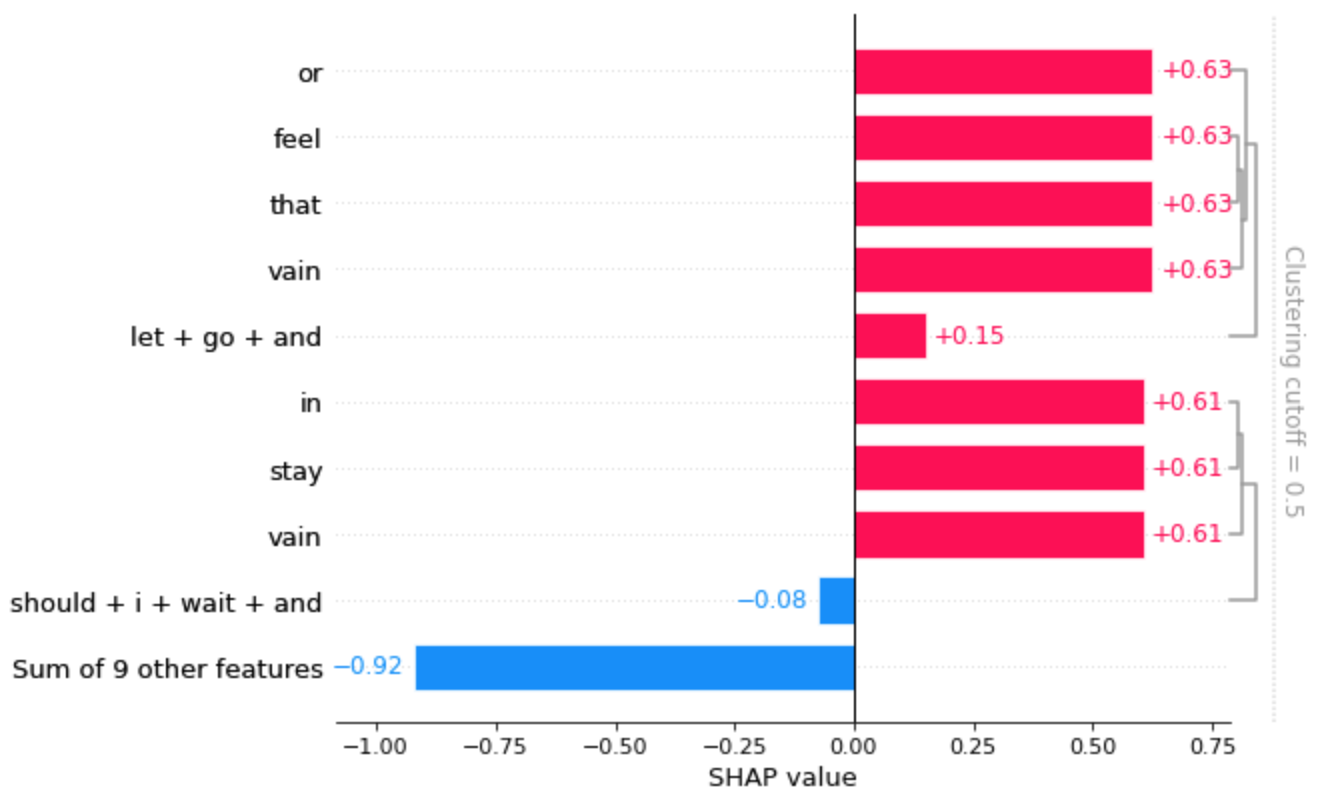
shap.plots.barを使って棒グラフで可視化することもできます。
shap.plots.bar(shap_values[0,:,predict])
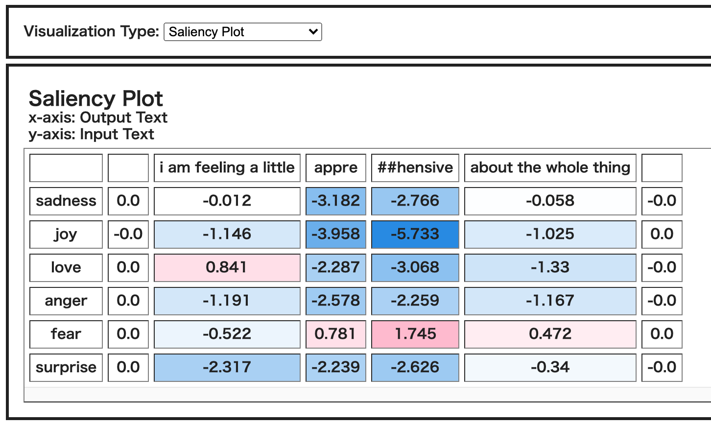
別の文章でも試してみます。ピックアップされた文章は「i am feeling a little apprehensive about the whole thing」でした。
DeepL翻訳「全体的に少し不安を感じています。」
正解ラベル、予測ラベルともに「fear」でした。
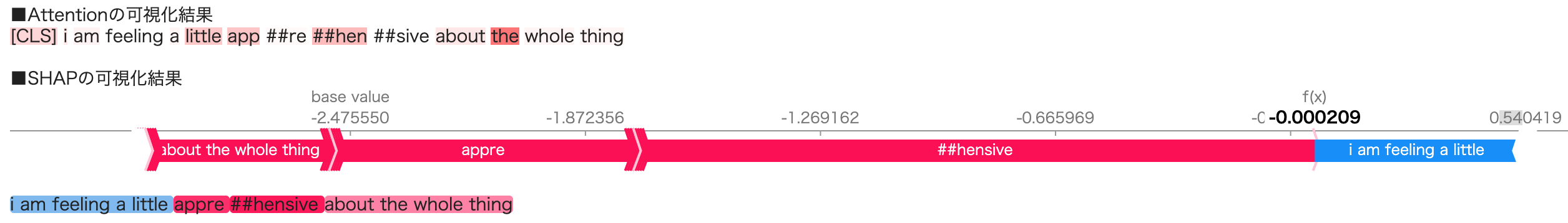
肝心の一番fearっぽい単語「apprehensive」がサブワードで分割されてしまってますが、Attentionもなんとか部分的にAttentionしてるようです。とはいえ、「the」に一番強くAttentionしてるのは微妙な気がします。それに対して、SHAPのほうでは、「apprehensive」全体がfearに強く効いたことが見受けられます。
※Attentionの結果とSHAPの結果で「apprehensive」の分割のされ方が異なるようにみられます。(SHAPのほうでは「app ##re」ではなく「appre」とくっついている)
これはshap.plots.textが裏でSHAP値が近い場合は単語をグルーピング処理をしているため、のようです。どれくらいSHAP値が似ていれば単語をグループ化するかの閾値はgroup_thresholdで指定できます。
ちなみに今回のケースは「app」と「##re」のSHAP値は同じでした。
詳しくはReferenceをご参照ください。
heatmapや棒グラフの可視化結果は以下のようになりました。

複数文章に対して適用してみる
公式リファレンスでやってるみたいに、複数の文章のSHAP値をまとめて計算して、SHAP値を可視化することで、特定のラベルによく効く単語を調べてみようと思います。そのラベルの重要語の抽出といったところでしょうか。
# 予測が正しかった文章のみを抽出したいので、テストデータの各文章に対して予測ラベルを付与しておく
predict_list = []
for i in range(0, len(test_df), 10):
    _s = test_df['text'][i:i+10]
    predict_list += f(_s).argmax(dim=1).tolist()
test_df['pred'] = predict_list
# ちなみにこの予測結果と上でF1-scoreを算出したときの結果は微妙に異なります。
# 上で算出したときはpaddingはtorchtextが行った結果を使っており、ミニバッチ毎のmax_lengthでpaddingされていたかと思いますが、
# こちらで算出した結果は、全文章に対してmax_length 128でpaddingして(全文章の長さがpadding込みで128になって)おり、
# classifierに通すデータが異なっているのが原因と思われます。
# とりあえず細かいことは気にしない精神で実装してます、ご容赦いただけたらと思います。。。
loveと予測した文章全てのSHAP値を計算してみます。
target_label = "love"
label_id = label2id[target_label]
sentences = test_df.query('pred == @label_id')['text']

# ぼちぼち時間かかります。
shap_values = explainer(sentences)
SHAP値の高い順番に可視化してみます。max_displayで省略しない件数を指定できます。
shap.plots.bar(shap_values[:,:,'love'].mean(0), max_display=10)
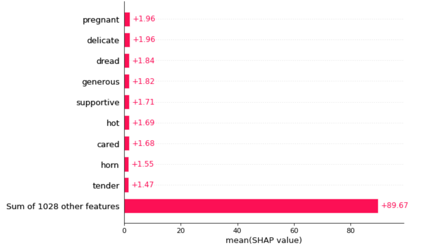
「pregnant(妊娠中)」が一番上にきてるあたりそれっぽいですが、なんとなくデータのバイアスを感じなくもない。
angerでも試してみます。
target_label = "anger"
label_id = label2id[target_label]
sentences = test_df.query('pred == @label_id')['text']

shap_values = explainer(sentences)

# SHAP値の高い順番に可視化してみる。
shap.plots.bar(shap_values[:,:,'anger'].mean(0), max_display=10)
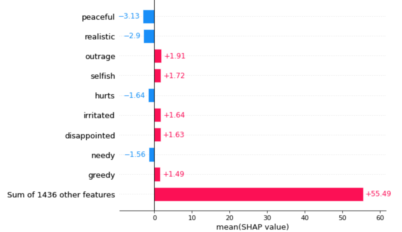
「peaceful(平和)」が一番マイナス方向に効いたってことでとてもそれっぽい結果です。「outrage(怒り、暴力)」がangerによく効く単語となっているのもいい感じな結果です。
おわりに
自然言語処理に対するSHAPの使い方がちょっとだけわかった気に慣れました。
正直まだまだSHAPの使い方がよくわかっていないところがありますが、今回使ってみて、AttentionよりもSHAPの可視化結果のほうがそれっぽく感じます。
やっぱり説明性とかのトピックは面白い
おわり