きっかけ

メタ学習やグラフニューラルネットワーク、事前知識としての利用を含む知識構造の利用、知識保存、オントロジー、因果推論に興味あり。
関連し、ベイジアンネットワークを手軽に実装できないかとライブラリを探していた。
pgmpyがよさそうであったので、一通りの流れを記録しておく。

pgmpy：pgmpy is a python library for working with Probabilistic Graphical Models.
https://pgmpy.org/

参考

Titanicデータでベイジアンネットワークを実装
https://qiita.com/YuyaOmori/items/e051f0360d1f9562620b

ベイジアンネットワーク：入門からヒューマンモデリングへの応用まで
https://staff.aist.go.jp/y.motomura/paper/BSJ0403.pdf

環境

Windows10
Python3.7
Anaconda
pgmpy==0.1.9

インストール

pip install pgmpy==0.1.9

pytorchを入れておらずnonGPUならば

conda install pytorch torchvision cpuonly -c pytorch

データ

次の離散データを使用。

import pandas as pd
df = pd.DataFrame()
df['t'] = [1, 1, 1, 1, 0, 0, 1, 1, 1, 2, 0, 0, 1, 1, 1, 2, 2, 2, 2, 2] #3分類
df['a'] = [2, 2, 2, 2, 1, 1, 1, 1, 2, 1, 1, 2, 0, 0, 0, 1, 1, 2, 2, 2] #3分類
df['h'] = [0, 0, 0, 1, 0, 0, 1, 1, 1, 1, 0, 0, 0, 1, 1, 1, 1, 1, 1, 1] #2分類

実行

モデル構造の定義

from pgmpy.models import BayesianModel
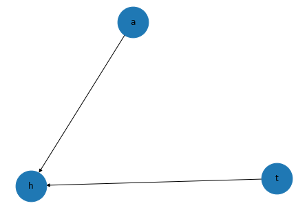
model = BayesianModel([('t','h'),('a','h')])

t→h、a→hの有向非巡回グラフとした。

モデル内にCPD作成・確認

model.fit(df) #条件は省略。標準ではオーバーフィットに特に注意

print(model.get_cpds('t'))
print(model.get_cpds('a'))
print(model.get_cpds('h'))

出力

+------+-----+
| t(0) | 0.2 |
+------+-----+
| t(1) | 0.5 |
+------+-----+
| t(2) | 0.3 |
+------+-----+
+------+------+
| a(0) | 0.15 |
+------+------+
| a(1) | 0.4  |
+------+------+
| a(2) | 0.45 |
+------+------+
+------+------+--------------------+------+------+------+------+------+------+------+
| a    | a(0) | a(0)               | a(0) | a(1) | a(1) | a(1) | a(2) | a(2) | a(2) |
+------+------+--------------------+------+------+------+------+------+------+------+
| t    | t(0) | t(1)               | t(2) | t(0) | t(1) | t(2) | t(0) | t(1) | t(2) |
+------+------+--------------------+------+------+------+------+------+------+------+
| h(0) | 0.5  | 0.3333333333333333 | 0.5  | 1.0  | 0.0  | 0.0  | 1.0  | 0.6  | 0.0  |
+------+------+--------------------+------+------+------+------+------+------+------+
| h(1) | 0.5  | 0.6666666666666666 | 0.5  | 0.0  | 1.0  | 1.0  | 0.0  | 0.4  | 1.0  |
+------+------+--------------------+------+------+------+------+------+------+------+

推論１

from pgmpy.inference import VariableElimination
ve = VariableElimination(model)

#t=1,h=1とした場合のaは？
print(ve.map_query(variables=['a'], evidence={'t':1, 'h':1}))

出力

{'a': 1}

推論２

#t=0,1,2とした場合のa,hは？
for i in [0,1,2]:
    print(ve.query(variables=['a', 'h'], evidence={'t':i}))

出力


+------+------+------------+
| a    | h    |   phi(a,h) |
+======+======+============+
| a(0) | h(0) |     0.0750 |
+------+------+------------+
| a(0) | h(1) |     0.0750 |
+------+------+------------+
| a(1) | h(0) |     0.4000 |
+------+------+------------+
| a(1) | h(1) |     0.0000 |
+------+------+------------+
| a(2) | h(0) |     0.4500 |
+------+------+------------+
| a(2) | h(1) |     0.0000 |
+------+------+------------+

+------+------+------------+
| h    | a    |   phi(h,a) |
+======+======+============+
| h(0) | a(0) |     0.0500 |
+------+------+------------+
| h(0) | a(1) |     0.0000 |
+------+------+------------+
| h(0) | a(2) |     0.2700 |
+------+------+------------+
| h(1) | a(0) |     0.1000 |
+------+------+------------+
| h(1) | a(1) |     0.4000 |
+------+------+------------+
| h(1) | a(2) |     0.1800 |
+------+------+------------+

+------+------+------------+
| a    | h    |   phi(a,h) |
+======+======+============+
| a(0) | h(0) |     0.0750 |
+------+------+------------+
| a(0) | h(1) |     0.0750 |
+------+------+------------+
| a(1) | h(0) |     0.0000 |
+------+------+------------+
| a(1) | h(1) |     0.4000 |
+------+------+------------+
| a(2) | h(0) |     0.0000 |
+------+------+------------+
| a(2) | h(1) |     0.4500 |
+------+------+------------+

補足

model.fit(df) は、例えば、次に分割できる。
分割したほうが扱いやすいこともあろうかとメモ。

#CPD作成部分
from pgmpy.estimators import BayesianEstimator
estimator = BayesianEstimator(model, df)
cpd_ta = estimator.estimate_cpd('t', prior_type='dirichlet', pseudo_counts=[[0],[0],[0]])
cpd_aa = estimator.estimate_cpd('a', prior_type='dirichlet', pseudo_counts=[[0],[0],[0]])
cpd_h = estimator.estimate_cpd('h', prior_type='dirichlet', pseudo_counts=[[0,0,0,0,0,0,0,0,0],[0,0,0,0,0,0,0,0,0]])

#CPD入力部分
model.add_cpds(cpd_ta, cpd_aa, cpd_h)

CPDを任意に作成する場合には、例えば、次とする。

from pgmpy.factors.discrete import TabularCPD
cpd_h = TabularCPD(variable='h', variable_card=2,
                        values=[[1, 0.3, 0.5, 1, 0, 0, 1, 0.6, 0],
                                [0, 0.7, 0.5, 0, 1, 1, 0, 0.4, 1]],
                        evidence=['t', 'a'],
                        evidence_card=[3, 3])

構造学習については省略する。
multiply connectedに対応したJunction treeのような機能もあるようだ。どこまでできるのか確認中。
時系を考慮した動的ベイジアンネットワークという手法もあるそうだ。
【リレー連載】わたしの推しノード –隠れた関係を見つける名探偵「ベイズノード」が変数間の因果構造を解き明かす
https://www.ibm.com/blogs/solutions/jp-ja/spssmodeler-push-node-18/
参考としirisデータセットで試行。構造学習において特徴の一つが現れず困ったが他は問題なし。
個の抽出を重視したい。次は以下を進める。
階層ベイズ（「ベイズモデリングの世界」から）
https://recruit.cct-inc.co.jp/tecblog/machine-learning/hierarchical-bayesian/
PyMC3。python3.6未満でしか動作しないTheano必要。
＊PyMC4待ち→開発中止?。代わりにPyMC3 v3.10.0 (7 December 2020)がTheanoからJAXにバックエンドを変更して登場。
　https://github.com/pymc-devs/pymc4/tree/1c5e23825271fc2ff0c701b9224573212f56a534
＊Pythonで体験するベイズ推論:PyMCによるMCMC入門
　https://github.com/CamDavidsonPilon/Probabilistic-Programming-and-Bayesian-Methods-for-Hackers
　PyMC2を触ったのだが、ほぼ忘れている。
切り替え時かな
NumPyroに階層ベイズあり。PyTorchをベースにしたpyroもほぼ同じようだ。
https://pyro.ai/numpyro/bayesian_hierarchical_linear_regression.html#2.-Modelling:-Bayesian-Hierarchical-Linear-Regression-with-Partial-Pooling
https://qiita.com/takeajioka/items/ab299d75efa184eb1432

＊【ネットワークの統計解析】第5回代表的なネットワークのモデルを俯瞰する (3)
https://buildersbox.corp-sansan.com/entry/2021/02/19/114000

＊セミパラメトリックアプローチによる統計的因果探索
https://www.jstage.jst.go.jp/article/jsaifpai/118/0/118_02/_article/-char/ja/

＊Symbolic Knowledge Distillation: from General Language Models to Commonsense Models
https://arxiv.org/abs/2110.07178
GPT-3 から常識抽出，知識グラフを作成

＊ベイジアンネットワークによる定位放射線治療後の転帰の予測
https://drive.google.com/file/d/1D1bEiuddl-iqjWuDUU1zj5KQ5eApKnFI/view
1次元にまとめた評価基準における他の機械学習手段の結果との比較はともかくとして，ベイジアンネットワークの結果は臨床感覚に近かったとのこと．
自分はBERT荷違和感をおぼえることがたまにあるが，分布の適正さと感覚に関連があると考えればそうなのだろう．

＊バックドア基準
https://youtu.be/AqifHlVi6LE

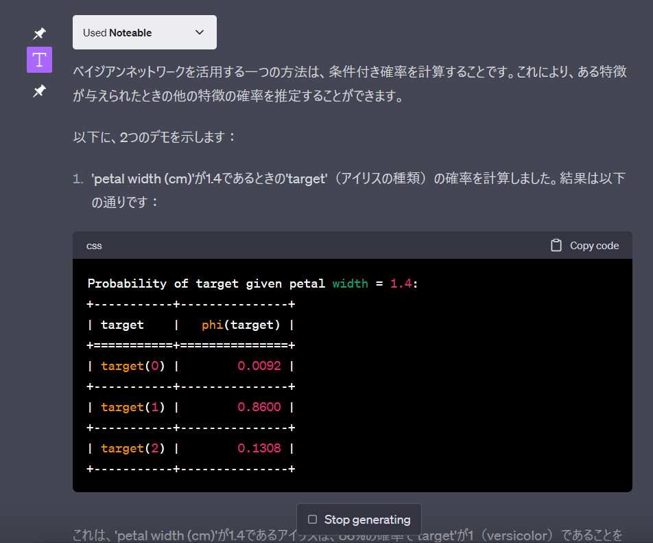
ChatGPT plugin noteableを用い，irisデータから構造学習しネットワークを予測させた上で，ベイジアンネットワークを作成させてみた

次のツイートをみて興味深かったため，ベイジアンネットワークまでやらせてみた

ChatGPT+Noteableが超絶便利だったので、Irisデータセットを分析させてみる。標準統計量、ペアプロット、5つの予想モデル作成、次元削減&クラスタリングとベタな分析notebookが会話していくだけ一瞬で出来上がって、やはり超便利だった。データ分析の初手が変わってきそう!!1https://t.co/u3XuKTTXMX pic.twitter.com/1VvJOar8Vh
— セコン (@hotchpotch) May 27, 2023

で，

詳細はこちら

・・・いやはや・・・

ChatGPT追記） pgmpy：離散ベイジアンネットワークの試用 -推論まで

きっかけ

参考

環境

インストール

データ

実行

モデル構造の定義

モデル内にCPD作成・確認

推論１

推論２

補足

ChatGPT plugin noteableを用い，irisデータから構造学習しネットワークを予測させた上で，ベイジアンネットワークを作成させてみた

ChatGPT追記）　pgmpy：離散ベイジアンネットワークの試用 -推論まで