This is an English translation of 実装技術者向けB-スプライン曲線入門.
Introduction
This article provides a comprehensive guide to implementing B-spline curves. It includes the derivation process and implementation examples for converting to Bézier curves and drawing them. The following three types1 of uniform(*) B-spline curves, degree 3, are included. NURBS is not included.
| Open | Closed | Clamped |
|---|---|---|
 |
 |
 |
(*) Clamped B-spline curves are sometimes considered non-uniform because multiple knots are contained in their knot vectors, but since the multiple knots are at begin or end of the knot vectors, not at middle. So it is considered uniform in this article. (whether they are at middle or at begin/end makes a significant difference)
Definition of B-Spline Curves
B-spline curves is a parametric curve expressed as an nth-order function of the parametric variable (or parameter) $t$. The $x$ and $y$ coordinates of each control point are multiplied by basis functions, which is an nth-order function of $t$, to obtain $x$ and $y$ coordinates on the curve.
If the degree $n$ is $3$ and the number of control points is $m$ ($m \geq n+1$), then:
\begin{array}{ll}
x=f(t)=b_{0,3}(t)P_{0_x}+b_{1,3}(t)P_{1_x}+ \dots +b_{m-1,3}(t)P_{{m-1}_x} \\
y=g(t)=b_{0,3}(t)P_{0_y}+b_{1,3}(t)P_{1_y}+ \dots +b_{m-1,3}(t)P_{{m-1}_y}
\end{array}
$b_{0,3}(t)$ to $b_{m-1,3}(t)$ are basis functions.
Let $[f(t),g(t)]=\boldsymbol{S}(t)$ and $[P_{i_x},P_{i_y}]=\boldsymbol{P}_i$, and we obtain the following Bernstein representation.
\boldsymbol{S}(t)=\sum_{i=0}^{m-1}b_{i,n}(t)\boldsymbol{P}_i
The basis functions of B-spline curve are defined by "de Boor-Cox recursion formula".
\begin{align}
&b_{i,0}(t) =
\left
\{
\begin{array}{ll}
1 & if \quad t_i \leq t < t_{i+1} \\
0 & otherwise
\end{array}
\right. \\
&b_{i,k}(t) =
\frac{t-t_i}{t_{i+k}-t_i} b_{i,k-1}(t) +
\frac{t_{i+k+1}-t}{t_{i+k+1}-t_{i+1}}  b_{i+1,k-1}(t)
\end{align}
Where $t_i$ is a knot vector, a sequence of $m+n+1$ numbers. The characteristics of the curve can be adjusted by the knot vector.
The knot vector of a basic uniform B-spline curve is a uniformly spaced numbers. Below is an example of a knot vector for $n=3$ and $m=4$.
\begin{bmatrix} t_0 & t_1 & t_2 & t_3 & t_4 & t_5 & t_6 & t_7 \end{bmatrix} = \begin{bmatrix} 0 & 1 & 2 & 3 & 4 & 5 & 6 & 7 \end{bmatrix}
An example of the basis functions and curve for this knot vector is as follows. The range of $t$ is $3 \leq t < 4$. The start and end points of the curve does not overlap any control points.


The relationship between knot vector, basis function, and control point is shown in the diagram below.2
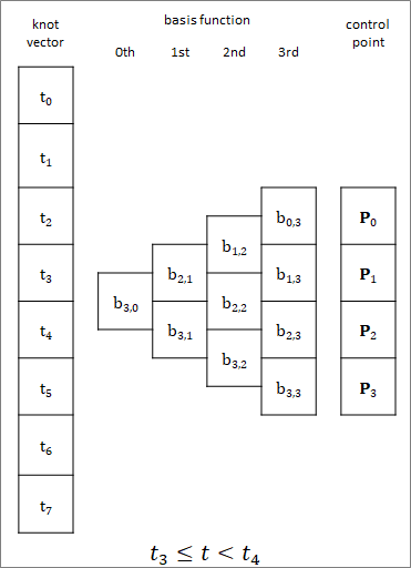
When $t_3 \leq t < t_4$, the 0th $b_{3,0}$ becomes 1, and the 1st $b_{2,1}$ to $b_{3,1}$, the 2nd $b_{1,2}$ to $b_{3,2}$, and the 3rd $b_{0,3}$ to $b_{3,3}$ are determined sequentially. The valid elements form a triangular array as shown in above.
No calculation is necessary for elements other than the triangular array. Also, no calculation is necessary for terms that refer to other elements.
Manipulating Knot Vector
Parameter range can be changed
Since the calculation of the recurrence formula involves the difference and ratio between knots, we can arbitrarily change the range of $t$ by adding or multiplying a constant to the entire knot vector. Followings are for the same curve.
| Knot Vector | Range of $t$ |
|---|---|
| $ \begin{bmatrix} 0 & 1 & 2 & 3 & 4 & 5 & 6 & 7 \end{bmatrix} $ | $3\leq t<4$ |
| $ \begin{bmatrix} -3 & -2 & -1 & 0 & 1 & 2 & 3 & 4 \end{bmatrix} $ | $0\leq t<1$ |
| $ \begin{bmatrix} 0 & 0.5 & 1 & 1.5 & 2 & 2.5 & 3 & 3.5 \end{bmatrix} $ | $1.5\leq t<2$ |
Knots at both ends are arbitrary
The elements at both ends of the knot vector ($t_0$ and $t_7$ in above example) are not used in calculating the basis functions. They may be arbitrary values.
Expansion of Basis Function
Below is Sage Math notebook for expansion of B-spline basis function to polynomial. From the result, we can see that $b_{2,1}$ to $b_{3,1}$ are linear functions of $t$, $b_{1,2}$ to $b_{3,2}$ are quadratic functions of $t$, and $b_{0,3}$ to $b_{3,3}$ are cubic functions of $t$. The coefficients of each term vary depending on the knot vector.
var ('t')
tk=[-3, -2, -1, 0, 1, 2, 3, 4]
b30=1
b21=                            (tk[4]-t)/(tk[4]-tk[3])*b30
b31=(t-tk[3])/(tk[4]-tk[3])*b30
b12=                            (tk[4]-t)/(tk[4]-tk[2])*b21
b22=(t-tk[2])/(tk[4]-tk[2])*b21+(tk[5]-t)/(tk[5]-tk[3])*b31
b32=(t-tk[3])/(tk[5]-tk[3])*b31
b03=                            (tk[4]-t)/(tk[4]-tk[1])*b12
b13=(t-tk[1])/(tk[4]-tk[1])*b12+(tk[5]-t)/(tk[5]-tk[2])*b22
b23=(t-tk[2])/(tk[5]-tk[2])*b22+(tk[6]-t)/(tk[6]-tk[3])*b32
b33=(t-tk[3])/(tk[6]-tk[3])*b32
b21.simplify_full()
b31.simplify_full()
b12.simplify_full()
b22.simplify_full()
b32.simplify_full()
b03.simplify_full()
b13.simplify_full()
b23.simplify_full()
b33.simplify_full()
-t + 1
t
1/2*t^2 - t + 1/2
-t^2 + t + 1/2
1/2*t^2
-1/6*t^3 + 1/2*t^2 - 1/2*t + 1/6
1/2*t^3 - t^2 + 2/3
-1/2*t^3 + 1/2*t^2 + 1/2*t + 1/6
1/6*t^3
Using $b_{0,3}$ to $b_{3,3}$ of the expanded polynomials, B-spline curves can be expressed in following matrix form, where $\boldsymbol{R_{bsp}}$ is "coefficient matrix".
\boldsymbol{S}(t)=
\begin{bmatrix}
t^3 & t^2 & t & 1
\end{bmatrix}
\boldsymbol{R_{bsp}}
\begin{bmatrix}
{\boldsymbol{P}}_0 \\
{\boldsymbol{P}}_1 \\
{\boldsymbol{P}}_2 \\
{\boldsymbol{P}}_3
\end{bmatrix}
\boldsymbol{R_{bsp}}=
\begin{bmatrix}
-\frac{1}{6} & \frac{1}{2} & -\frac{1}{2} & \frac{1}{6} \\
\frac{1}{2} & -1 & \frac{1}{2} & 0 \\
-\frac{1}{2} & 0 & \frac{1}{2} & 0 \\
\frac{1}{6} & \frac{2}{3} & \frac{1}{6} & 0
\end{bmatrix}
Increasing Control Points
We can arbitrarily increase the number of control points on B-spline curves without changing its degree. The number of knots also increases with the number of control points, causing the shape of triangular matrix of basis function to expand vertically. Following diagram is for increasing number of control points to five ($m=5$).
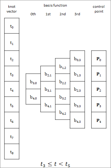
Below is an example of a knot vector:
$ \begin{bmatrix} 0 & 1 & 2 & 3 & 4 & 5 & 6 & 7 & 8 \end{bmatrix} $
Following basis functions and an example of curve is for above case. The graph of basis function is identical to $m=4$ graph repeating horizontally twice.


Dividing Curve
In the above case, the range of $t$ is $3 \leq t < 5$, but since only $b_{3,0}$ or $b_{4,0}$ can be 1 at a time, only four terms between $b_{0,3}$ and $b_{4,3}$ are valid (non-zero) at a time. Therefore, the control points relevant to determining the curve shape are $P_0$ to $P_3$ for $3 \leq t < 4$, and $P_1$ to $P_4$ for $4 \leq t < 5$. From this reason, a B-spline curve ($m=5$) can be considered of as a composite curve consisting of two curves (curve segments).
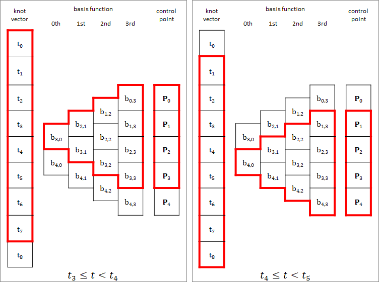
Therefore, we can divide the control points into two sets and draw the curve in two steps.
| Control points | Range of $t$ | Knot vector | |
|---|---|---|---|
| 0 | $ \begin{bmatrix} \boldsymbol{P}_0 & \boldsymbol{P}_1 & \boldsymbol{P}_2 & \boldsymbol{P}_3 \end{bmatrix} $ | $3\leq t<4$ | $ \begin{bmatrix} 0 & 1 & 2 & 3 & 4 & 5 & 6 & 7 \end{bmatrix} $ |
| 1 | $ \begin{bmatrix} \boldsymbol{P}_1 & \boldsymbol{P}_2 & \boldsymbol{P}_3 & \boldsymbol{P}_4 \end{bmatrix} $ | $4\leq t<5$ | $ \begin{bmatrix} 1 & 2 & 3 & 4 & 5 & 6 & 7 & 8 \end{bmatrix} $ |
By aligning the range of $t$, we can reuse the same knot vector.
| Control points | Range of $t$ | Knot vector | |
|---|---|---|---|
| 0 | $ \begin{bmatrix} \boldsymbol{P}_0 & \boldsymbol{P}_1 & \boldsymbol{P}_2 & \boldsymbol{P}_3 \end{bmatrix} $ | $0\leq t<1$ | $ \begin{bmatrix} -3 & -2 & -1 & 0 & 1 & 2 & 3 & 4 \end{bmatrix} $ |
| 1 | $ \begin{bmatrix} \boldsymbol{P}_1 & \boldsymbol{P}_2 & \boldsymbol{P}_3 & \boldsymbol{P}_4 \end{bmatrix} $ | $0\leq t<1$ | $ \begin{bmatrix} -3 & -2 & -1 & 0 & 1 & 2 & 3 & 4 \end{bmatrix} $ |
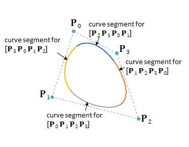
Closed B-Spline Curve
By using control points cyclically, we can draw closed B-spline curves.
| Control points | Range of $t$ | Knot vector | |
|---|---|---|---|
| 0 | $ \begin{bmatrix} \boldsymbol{P}_0 & \boldsymbol{P}_1 & \boldsymbol{P}_2 & \boldsymbol{P}_3 \end{bmatrix} $ | $0\leq t<1$ | $ \begin{bmatrix} -3 & -2 & -1 & 0 & 1 & 2 & 3 & 4 \end{bmatrix} $ |
| 1 | $ \begin{bmatrix} \boldsymbol{P}_1 & \boldsymbol{P}_2 & \boldsymbol{P}_3 & \boldsymbol{P}_0 \end{bmatrix} $ | $0\leq t<1$ | $ \begin{bmatrix} -3 & -2 & -1 & 0 & 1 & 2 & 3 & 4 \end{bmatrix} $ |
| 2 | $ \begin{bmatrix} \boldsymbol{P}_2 & \boldsymbol{P}_3 & \boldsymbol{P}_0 & \boldsymbol{P}_1 \end{bmatrix} $ | $0\leq t<1$ | $ \begin{bmatrix} -3 & -2 & -1 & 0 & 1 & 2 & 3 & 4 \end{bmatrix} $ |
| 3 | $ \begin{bmatrix} \boldsymbol{P}_3 & \boldsymbol{P}_0 & \boldsymbol{P}_1 & \boldsymbol{P}_2 \end{bmatrix} $ | $0\leq t<1$ | $ \begin{bmatrix} -3 & -2 & -1 & 0 & 1 & 2 & 3 & 4 \end{bmatrix} $ |
Clamped B-Spline Curve
If the first and last $n+1$ knots ($n$ is the degree) of the knot vector have the same value (multiple knots), start and end points of the curve overlap the control points, resulting a clamped B-spline curve.
Below is an example of knot vectors with $4 \leq m \leq 8$:
| $m$ | Knot vector |
|---|---|
| 4 | $ \begin{bmatrix} 0 & 0 & 0 & 0 & 1 & 1 & 1 & 1 \end{bmatrix} $ |
| 5 | $ \begin{bmatrix} 0 & 0 & 0 & 0 & 1 & 2 & 2 & 2 & 2 \end{bmatrix} $ |
| 6 | $ \begin{bmatrix} 0 & 0 & 0 & 0 & 1 & 2 & 3 & 3 & 3 & 3 \end{bmatrix} $ |
| 7 | $ \begin{bmatrix} 0 & 0 & 0 & 0 & 1 & 2 & 3 & 4 & 4 & 4 & 4 \end{bmatrix} $ |
| 8 | $ \begin{bmatrix} 0 & 0 & 0 & 0 & 1 & 2 & 3 & 4 & 5 & 5 & 5 & 5 \end{bmatrix} $ |
Dividing the control points and aligning the range of $t$, we get the following:
| $m$ | Control point | Range of $t$ | Knot vector |
|---|---|---|---|
| 4 | $ \begin{bmatrix} \boldsymbol{P}_0 & \boldsymbol{P}_1 & \boldsymbol{P}_2 & \boldsymbol{P}_3 \end{bmatrix} $ | $0\leq t<1$ | $ \begin{bmatrix} 0 & 0 & 0 & 0 & 1 & 1 & 1 & 1 \end{bmatrix} $ |
| 5 | $ \begin{bmatrix} \boldsymbol{P}_0 & \boldsymbol{P}_1 & \boldsymbol{P}_2 & \boldsymbol{P}_3 \end{bmatrix} $ | $0\leq t<1$ | $ \begin{bmatrix} 0 & 0 & 0 & 0 & 1 & 2 & 2 & 2 \end{bmatrix} $ |
| $ \begin{bmatrix} \boldsymbol{P}_1 & \boldsymbol{P}_2 & \boldsymbol{P}_3 & \boldsymbol{P}_4 \end{bmatrix} $ | $0\leq t<1$ | $ \begin{bmatrix} -1 & -1 & -1 & 0 & 1 & 1 & 1 & 1 \end{bmatrix} $ | |
| 6 | $ \begin{bmatrix} \boldsymbol{P}_0 & \boldsymbol{P}_1 & \boldsymbol{P}_2 & \boldsymbol{P}_3 \end{bmatrix} $ | $0\leq t<1$ | $ \begin{bmatrix} 0 & 0 & 0 & 0 & 1 & 2 & 3 & 3 \end{bmatrix} $ |
| $ \begin{bmatrix} \boldsymbol{P}_1 & \boldsymbol{P}_2 & \boldsymbol{P}_3 & \boldsymbol{P}_4 \end{bmatrix} $ | $0\leq t<1$ | $ \begin{bmatrix} -1 & -1 & -1 & 0 & 1 & 2 & 2 & 2 \end{bmatrix} $ | |
| $ \begin{bmatrix} \boldsymbol{P}_2 & \boldsymbol{P}_3 & \boldsymbol{P}_4 & \boldsymbol{P}_5 \end{bmatrix} $ | $0\leq t<1$ | $ \begin{bmatrix} -2 & -2 & -1 & 0 & 1 & 1 & 1 & 1 \end{bmatrix} $ | |
| 7 | $ \begin{bmatrix} \boldsymbol{P}_0 & \boldsymbol{P}_1 & \boldsymbol{P}_2 & \boldsymbol{P}_3 \end{bmatrix} $ | $0\leq t<1$ | $ \begin{bmatrix} 0 & 0 & 0 & 0 & 1 & 2 & 3 & 4 \end{bmatrix} $ |
| $ \begin{bmatrix} \boldsymbol{P}_1 & \boldsymbol{P}_2 & \boldsymbol{P}_3 & \boldsymbol{P}_4 \end{bmatrix} $ | $0\leq t<1$ | $ \begin{bmatrix} -1 & -1 & -1 & 0 & 1 & 2 & 3 & 3 \end{bmatrix} $ | |
| $ \begin{bmatrix} \boldsymbol{P}_2 & \boldsymbol{P}_3 & \boldsymbol{P}_4 & \boldsymbol{P}_5 \end{bmatrix} $ | $0\leq t<1$ | $ \begin{bmatrix} -2 & -2 & -1 & 0 & 1 & 2 & 2 & 2 \end{bmatrix} $ | |
| $ \begin{bmatrix} \boldsymbol{P}_3 & \boldsymbol{P}_4 & \boldsymbol{P}_5 & \boldsymbol{P}_6 \end{bmatrix} $ | $0\leq t<1$ | $ \begin{bmatrix} -3 & -2 & -1 & 0 & 1 & 1 & 1 & 1 \end{bmatrix} $ | |
| 8 | $ \begin{bmatrix} \boldsymbol{P}_0 & \boldsymbol{P}_1 & \boldsymbol{P}_2 & \boldsymbol{P}_3 \end{bmatrix} $ | $0\leq t<1$ | $ \begin{bmatrix} 0 & 0 & 0 & 0 & 1 & 2 & 3 & 4 \end{bmatrix} $ |
| $ \begin{bmatrix} \boldsymbol{P}_1 & \boldsymbol{P}_2 & \boldsymbol{P}_3 & \boldsymbol{P}_4 \end{bmatrix} $ | $0\leq t<1$ | $ \begin{bmatrix} -1 & -1 & -1 & 0 & 1 & 2 & 3 & 4 \end{bmatrix} $ | |
| $ \begin{bmatrix} \boldsymbol{P}_2 & \boldsymbol{P}_3 & \boldsymbol{P}_4 & \boldsymbol{P}_5 \end{bmatrix} $ | $0\leq t<1$ | $ \begin{bmatrix} -2 & -2 & -1 & 0 & 1 & 2 & 3 & 3 \end{bmatrix} $ | |
| $ \begin{bmatrix} \boldsymbol{P}_3 & \boldsymbol{P}_4 & \boldsymbol{P}_5 & \boldsymbol{P}_6 \end{bmatrix} $ | $0\leq t<1$ | $ \begin{bmatrix} -3 & -2 & -1 & 0 & 1 & 2 & 2 & 2 \end{bmatrix} $ | |
| $ \begin{bmatrix} \boldsymbol{P}_4 & \boldsymbol{P}_5 & \boldsymbol{P}_6 & \boldsymbol{P}_7 \end{bmatrix} $ | $0\leq t<1$ | $ \begin{bmatrix} -3 & -2 & -1 & 0 & 1 & 1 & 1 & 1 \end{bmatrix} $ |
The coefficient matrix $\boldsymbol{R_{bsp}}$ for each knot vector is as follows. The coefficient matrix $ \begin{bmatrix} \boldsymbol{P}_2 & \boldsymbol{P}_3 & \boldsymbol{P}_4 & \boldsymbol{P}_5 \end{bmatrix} $ for $m=8$ is equal to the coefficient matrix of open B-spline curve. For $m \ge 9$, this coefficient matrix is repeated as many times as necessary.3
| $m$ | Control point | $\boldsymbol{R_{bsp}}$ |
|---|---|---|
| 4 | $ \begin{bmatrix} \boldsymbol{P}_0 & \boldsymbol{P}_1 & \boldsymbol{P}_2 & \boldsymbol{P}_3 \end{bmatrix} $ | $ \begin{bmatrix} -1 && 3 && -3 && 1 \\ 3 && -6 && 3 && 0 \\ -3 && 3 && 0 && 0 \\ 1 && 0 && 0 && 0 \end{bmatrix} $ |
| 5 | $ \begin{bmatrix} \boldsymbol{P}_0 & \boldsymbol{P}_1 & \boldsymbol{P}_2 & \boldsymbol{P}_3 \end{bmatrix} $ | $ \begin{bmatrix} -1 && \frac{7}{4} && -1 && \frac{1}{4} \\ 3 && -\frac{9}{2} && \frac{3}{2} && 0 \\ -3 && 3 && 0 && 0 \\ 1 && 0 && 0 && 0 \end{bmatrix} $ |
| $ \begin{bmatrix} \boldsymbol{P}_1 & \boldsymbol{P}_2 & \boldsymbol{P}_3 & \boldsymbol{P}_4 \end{bmatrix} $ | $ \begin{bmatrix} -\frac{1}{4} && 1 && -\frac{7}{4} && 1 \\ \frac{3}{4} && -\frac{3}{2} && \frac{3}{4} && 0 \\ -\frac{3}{4} && 0 && \frac{3}{4} && 0 \\ \frac{1}{4} && \frac{1}{2} && \frac{1}{4} && 0 \end{bmatrix} $ | |
| 6 | $ \begin{bmatrix} \boldsymbol{P}_0 & \boldsymbol{P}_1 & \boldsymbol{P}_2 & \boldsymbol{P}_3 \end{bmatrix} $ | $ \begin{bmatrix} -1 && \frac{7}{4} && -\frac{11}{12} && \frac{1}{6} \\ 3 && -\frac{9}{2} && \frac{3}{2} && 0 \\ -3 && 3 && 0 && 0 \\ 1 && 0 && 0 && 0 \end{bmatrix} $ |
| $ \begin{bmatrix} \boldsymbol{P}_1 & \boldsymbol{P}_2 & \boldsymbol{P}_3 & \boldsymbol{P}_4 \end{bmatrix} $ | $ \begin{bmatrix} -\frac{1}{4} && \frac{7}{12} && -\frac{7}{12} && \frac{1}{4} \\ \frac{3}{4} && -\frac{5}{4} && \frac{1}{2} && 0 \\ -\frac{3}{4} && \frac{1}{4} && \frac{1}{2} && 0 \\ \frac{1}{4} && \frac{7}{12} && \frac{1}{6} && 0 \end{bmatrix} $ | |
| $ \begin{bmatrix} \boldsymbol{P}_2 & \boldsymbol{P}_3 & \boldsymbol{P}_4 & \boldsymbol{P}_5 \end{bmatrix} $ | $ \begin{bmatrix} -\frac{1}{6} && \frac{11}{12} && -\frac{7}{4} && 1 \\ \frac{1}{2} && -\frac{5}{4} && \frac{3}{4} && 0 \\ -\frac{1}{2} && -\frac{1}{4} && \frac{3}{4} && 0 \\ \frac{1}{6} && \frac{7}{12} && \frac{1}{4} && 0 \end{bmatrix} $ | |
| 7 | $ \begin{bmatrix} \boldsymbol{P}_0 & \boldsymbol{P}_1 & \boldsymbol{P}_2 & \boldsymbol{P}_3 \end{bmatrix} $ | $ \begin{bmatrix} -1 && \frac{7}{4} && -\frac{11}{12} && \frac{1}{6} \\ 3 && -\frac{9}{2} && \frac{3}{2} && 0 \\ -3 && 3 && 0 && 0 \\ 1 && 0 && 0 && 0 \end{bmatrix} $ |
| $ \begin{bmatrix} \boldsymbol{P}_1 & \boldsymbol{P}_2 & \boldsymbol{P}_3 & \boldsymbol{P}_4 \end{bmatrix} $ | $ \begin{bmatrix} -\frac{1}{4} && \frac{7}{12} && -\frac{1}{2} && \frac{1}{6} \\ \frac{3}{4} && -\frac{5}{4} && \frac{1}{2} && 0 \\ -\frac{3}{4} && \frac{1}{4} && \frac{1}{2} && 0 \\ \frac{1}{4} && \frac{7}{12} && \frac{1}{6} && 0 \end{bmatrix} $ | |
| $ \begin{bmatrix} \boldsymbol{P}_2 & \boldsymbol{P}_3 & \boldsymbol{P}_4 & \boldsymbol{P}_5 \end{bmatrix} $ | $ \begin{bmatrix} -\frac{1}{6} && \frac{1}{2} && -\frac{7}{12} && \frac{1}{4} \\ \frac{1}{2} && -1 && \frac{1}{2} && 0 \\ -\frac{1}{2} && 0 && \frac{1}{2} && 0 \\ \frac{1}{6} && \frac{2}{3} && \frac{1}{6} && 0 \end{bmatrix} $ | |
| $ \begin{bmatrix} \boldsymbol{P}_3 & \boldsymbol{P}_4 & \boldsymbol{P}_5 & \boldsymbol{P}_6 \end{bmatrix} $ | $ \begin{bmatrix} -\frac{1}{6} && \frac{11}{12} && -\frac{7}{4} && 1 \\ \frac{1}{2} && -\frac{5}{4} && \frac{3}{4} && 0 \\ -\frac{1}{2} && -\frac{1}{4} && \frac{3}{4} && 0 \\ \frac{1}{6} && \frac{7}{12} && \frac{1}{4} && 0 \end{bmatrix} $ | |
| 8 | $ \begin{bmatrix} \boldsymbol{P}_0 & \boldsymbol{P}_1 & \boldsymbol{P}_2 & \boldsymbol{P}_3 \end{bmatrix} $ | $ \begin{bmatrix} -1 && \frac{7}{4} && -\frac{11}{12} && \frac{1}{6} \\ 3 && -\frac{9}{2} && \frac{3}{2} && 0 \\ -3 && 3 && 0 && 0 \\ 1 && 0 && 0 && 0 \end{bmatrix} $ |
| $ \begin{bmatrix} \boldsymbol{P}_1 & \boldsymbol{P}_2 & \boldsymbol{P}_3 & \boldsymbol{P}_4 \end{bmatrix} $ | $ \begin{bmatrix} -\frac{1}{4} && \frac{7}{12} && -\frac{1}{2} && \frac{1}{6} \\ \frac{3}{4} && -\frac{5}{4} && \frac{1}{2} && 0 \\ -\frac{3}{4} && \frac{1}{4} && \frac{1}{2} && 0 \\ \frac{1}{4} && \frac{7}{12} && \frac{1}{6} && 0 \end{bmatrix} $ | |
| $ \begin{bmatrix} \boldsymbol{P}_2 & \boldsymbol{P}_3 & \boldsymbol{P}_4 & \boldsymbol{P}_5 \end{bmatrix} $ | $ \begin{bmatrix} -\frac{1}{6} && \frac{1}{2} && -\frac{1}{2} && \frac{1}{6} \\ \frac{1}{2} && -1 && \frac{1}{2} && 0 \\ -\frac{1}{2} && 0 && \frac{1}{2} && 0 \\ \frac{1}{6} && \frac{2}{3} && \frac{1}{6} && 0 \end{bmatrix} $ | if $m \ge 9$, repeat as many times as necessary. |
| $ \begin{bmatrix} \boldsymbol{P}_3 & \boldsymbol{P}_4 & \boldsymbol{P}_5 & \boldsymbol{P}_6 \end{bmatrix} $ | $ \begin{bmatrix} -\frac{1}{6} && \frac{1}{2} && -\frac{7}{12} && \frac{1}{4} \\ \frac{1}{2} && -1 && \frac{1}{2} && 0 \\ -\frac{1}{2} && 0 && \frac{1}{2} && 0 \\ \frac{1}{6} && \frac{2}{3} && \frac{1}{6} && 0 \end{bmatrix} $ | |
| $ \begin{bmatrix} \boldsymbol{P}_4 & \boldsymbol{P}_5 & \boldsymbol{P}_6 & \boldsymbol{P}_7 \end{bmatrix} $ | $ \begin{bmatrix} -\frac{1}{6} && \frac{11}{12} && -\frac{7}{4} && 1 \\ \frac{1}{2} && -\frac{5}{4} && \frac{3}{4} && 0 \\ -\frac{1}{2} && -\frac{1}{4} && \frac{3}{4} && 0 \\ \frac{1}{6} && \frac{7}{12} && \frac{1}{4} && 0 \end{bmatrix} $ |
Below is an example of a clamped B-spline curve with $m=5$.

Converting B-spline curve to a Bézier curve
Matrix form for a Bézier curve is as follows4:
\boldsymbol{B}(t)=
\begin{bmatrix}
t^3 & t^2 & t & 1
\end{bmatrix}
\boldsymbol{R_{bz}}
\begin{bmatrix}
{\boldsymbol{P_{bz}}}_0 \\
{\boldsymbol{P_{bz}}}_1 \\
{\boldsymbol{P_{bz}}}_2 \\
{\boldsymbol{P_{bz}}}_3
\end{bmatrix}
\boldsymbol{R_{bz}}=
\begin{bmatrix}
-1 & 3 & -3 & 1 \\
3 & -6 & 3 & 0 \\
-3 & 3 & 0 & 0 \\
1 & 0 & 0 & 0
\end{bmatrix}
A set of Bézier curve control points that is equivalent to B-spline curve can be obtained by following steps.
The Bézier curve is equivalent to the B-spline curve, so:
\boldsymbol{B}(t)=
\boldsymbol{S}(t)
and
\boldsymbol{R_{bz}}
\begin{bmatrix}
{\boldsymbol{P_{bz}}}_0 \\
{\boldsymbol{P_{bz}}}_1 \\
{\boldsymbol{P_{bz}}}_2 \\
{\boldsymbol{P_{bz}}}_3
\end{bmatrix}
=
\boldsymbol{R_{bsp}}
\begin{bmatrix}
{\boldsymbol{P}}_0 \\
{\boldsymbol{P}}_1 \\
{\boldsymbol{P}}_2 \\
{\boldsymbol{P}}_3
\end{bmatrix}
Multiplying by $\boldsymbol{R_{bz}}^{-1}$ from the left gives:
\begin{bmatrix}
{\boldsymbol{P_{bz}}}_0 \\
{\boldsymbol{P_{bz}}}_1 \\
{\boldsymbol{P_{bz}}}_2 \\
{\boldsymbol{P_{bz}}}_3
\end{bmatrix}
=
\boldsymbol{R_{bz}}^{-1}
\boldsymbol{R_{bsp}}
\begin{bmatrix}
{\boldsymbol{P_{bsp}}}_0 \\
{\boldsymbol{P_{bsp}}}_1 \\
{\boldsymbol{P_{bsp}}}_2 \\
{\boldsymbol{P_{bsp}}}_3
\end{bmatrix}
Applying the coefficient matrix of open B-spline curve to $\boldsymbol{R_{bsp}}$, we get "conversion matrix":
\boldsymbol{R_{bz}}^{-1}
\boldsymbol{R_{bsp}}=
\frac{1}{6}
\begin{bmatrix}
1 & 4 & 1 & 0 \\
0 & 4 & 2 & 0 \\
0 & 2 & 4 & 0 \\
0 & 1 & 4 & 1
\end{bmatrix}
Below is an example of converted control points for Bézier curve. Blue are control points for B-spline curve, and red are converted control points for Bézier curve.


Conversion matrices for clamped B-spline curves are as follows.
Since a clamped B-spline curve with $m=4$ is equivalent to a Bézier curve, the conversion matrix is identity matrix.
| $m$ | Control point | Conversion matrix |
|---|---|---|
| 4 | $ \begin{bmatrix} \boldsymbol{P}_0 & \boldsymbol{P}_1 & \boldsymbol{P}_2 & \boldsymbol{P}_3 \end{bmatrix} $ | $ \begin{bmatrix} 1 && 0 && 0 && 0 \\ 0 && 1 && 0 && 0 \\ 0 && 0 && 1 && 0 \\ 0 && 0 && 0 && 1 \end{bmatrix} $ |
| 5 | $ \begin{bmatrix} \boldsymbol{P}_0 & \boldsymbol{P}_1 & \boldsymbol{P}_2 & \boldsymbol{P}_3 \end{bmatrix} $ | $ \begin{bmatrix} 1 && 0 && 0 && 0 \\ 0 && 1 && 0 && 0 \\ 0 && \frac{1}{2} && \frac{1}{2} && 0 \\ 0 && \frac{1}{4} && \frac{1}{2} && \frac{1}{4} \end{bmatrix} $ |
| $ \begin{bmatrix} \boldsymbol{P}_1 & \boldsymbol{P}_2 & \boldsymbol{P}_3 & \boldsymbol{P}_4 \end{bmatrix} $ | $ \begin{bmatrix} \frac{1}{4} && \frac{1}{2} && \frac{1}{4} && 0 \\ 0 && \frac{1}{2} && \frac{1}{2} && 0 \\ 0 && 0 && 1 && 0 \\ 0 && 0 && 0 && 1 \end{bmatrix} $ | |
| 6 | $ \begin{bmatrix} \boldsymbol{P}_0 & \boldsymbol{P}_1 & \boldsymbol{P}_2 & \boldsymbol{P}_3 \end{bmatrix} $ | $ \begin{bmatrix} 1 && 0 && 0 && 0 \\ 0 && 1 && 0 && 0 \\ 0 && \frac{1}{2} && \frac{1}{2} && 0 \\ 0 && \frac{1}{4} && \frac{7}{12} && \frac{1}{6} \end{bmatrix} $ |
| $ \begin{bmatrix} \boldsymbol{P}_1 & \boldsymbol{P}_2 & \boldsymbol{P}_3 & \boldsymbol{P}_4 \end{bmatrix} $ | $ \begin{bmatrix} \frac{1}{4} && \frac{7}{12} && \frac{1}{6} && 0 \\ 0 && \frac{2}{3} && \frac{1}{3} && 0 \\ 0 && \frac{1}{3} && \frac{2}{3} && 0 \\ 0 && \frac{1}{6} && \frac{7}{12} && \frac{1}{4} \end{bmatrix} $ | |
| $ \begin{bmatrix} \boldsymbol{P}_2 & \boldsymbol{P}_3 & \boldsymbol{P}_4 & \boldsymbol{P}_5 \end{bmatrix} $ | $ \begin{bmatrix} \frac{1}{6} && \frac{7}{12} && \frac{1}{4} && 0 \\ 0 && \frac{1}{2} && \frac{1}{2} && 0 \\ 0 && 0 && 1 && 0 \\ 0 && 0 && 0 && 1 \end{bmatrix} $ | |
| 7 | $ \begin{bmatrix} \boldsymbol{P}_0 & \boldsymbol{P}_1 & \boldsymbol{P}_2 & \boldsymbol{P}_3 \end{bmatrix} $ | $ \begin{bmatrix} 1 && 0 && 0 && 0 \\ 0 && 1 && 0 && 0 \\ 0 && \frac{1}{2} && \frac{1}{2} && 0 \\ 0 && \frac{1}{4} && \frac{7}{12} && \frac{1}{6} \end{bmatrix} $ |
| $ \begin{bmatrix} \boldsymbol{P}_1 & \boldsymbol{P}_2 & \boldsymbol{P}_3 & \boldsymbol{P}_4 \end{bmatrix} $ | $ \begin{bmatrix} \frac{1}{4} && \frac{7}{12} && \frac{1}{6} && 0 \\ 0 && \frac{2}{3} && \frac{1}{3} && 0 \\ 0 && \frac{1}{3} && \frac{2}{3} && 0 \\ 0 && \frac{1}{6} && \frac{2}{3} && \frac{1}{6} \end{bmatrix} $ | |
| $ \begin{bmatrix} \boldsymbol{P}_2 & \boldsymbol{P}_3 & \boldsymbol{P}_4 & \boldsymbol{P}_5 \end{bmatrix} $ | $ \begin{bmatrix} \frac{1}{6} && \frac{2}{3} && \frac{1}{6} && 0 \\ 0 && \frac{2}{3} && \frac{1}{3} && 0 \\ 0 && \frac{1}{3} && \frac{2}{3} && 0 \\ 0 && \frac{1}{6} && \frac{7}{12} && \frac{1}{4} \end{bmatrix} $ | |
| $ \begin{bmatrix} \boldsymbol{P}_3 & \boldsymbol{P}_4 & \boldsymbol{P}_5 & \boldsymbol{P}_6 \end{bmatrix} $ | $ \begin{bmatrix} \frac{1}{6} && \frac{7}{12} && \frac{1}{4} && 0 \\ 0 && \frac{1}{2} && \frac{1}{2} && 0 \\ 0 && 0 && 1 && 0 \\ 0 && 0 && 0 && 1 \end{bmatrix} $ | |
| 8 | $ \begin{bmatrix} \boldsymbol{P}_0 & \boldsymbol{P}_1 & \boldsymbol{P}_2 & \boldsymbol{P}_3 \end{bmatrix} $ | $ \begin{bmatrix} 1 && 0 && 0 && 0 \\ 0 && 1 && 0 && 0 \\ 0 && \frac{1}{2} && \frac{1}{2} && 0 \\ 0 && \frac{1}{4} && \frac{7}{12} && \frac{1}{6} \end{bmatrix} $ |
| $ \begin{bmatrix} \boldsymbol{P}_1 & \boldsymbol{P}_2 & \boldsymbol{P}_3 & \boldsymbol{P}_4 \end{bmatrix} $ | $ \begin{bmatrix} \frac{1}{4} && \frac{7}{12} && \frac{1}{6} && 0 \\ 0 && \frac{2}{3} && \frac{1}{3} && 0 \\ 0 && \frac{1}{3} && \frac{2}{3} && 0 \\ 0 && \frac{1}{6} && \frac{2}{3} && \frac{1}{6} \end{bmatrix} $ | |
| $ \begin{bmatrix} \boldsymbol{P}_2 & \boldsymbol{P}_3 & \boldsymbol{P}_4 & \boldsymbol{P}_5 \end{bmatrix} $ | $ \begin{bmatrix} \frac{1}{6} && \frac{2}{3} && \frac{1}{6} && 0 \\ 0 && \frac{2}{3} && \frac{1}{3} && 0 \\ 0 && \frac{1}{3} && \frac{2}{3} && 0 \\ 0 && \frac{1}{6} && \frac{2}{3} && \frac{1}{6} \end{bmatrix} $ | if $m \ge 9$, repeat as many times as necessary. |
| $ \begin{bmatrix} \boldsymbol{P}_3 & \boldsymbol{P}_4 & \boldsymbol{P}_5 & \boldsymbol{P}_6 \end{bmatrix} $ | $ \begin{bmatrix} \frac{1}{6} && \frac{2}{3} && \frac{1}{6} && 0 \\ 0 && \frac{2}{3} && \frac{1}{3} && 0 \\ 0 && \frac{1}{3} && \frac{2}{3} && 0 \\ 0 && \frac{1}{6} && \frac{7}{12} && \frac{1}{4} \end{bmatrix} $ | |
| $ \begin{bmatrix} \boldsymbol{P}_4 & \boldsymbol{P}_5 & \boldsymbol{P}_6 & \boldsymbol{P}_7 \end{bmatrix} $ | $ \begin{bmatrix} \frac{1}{6} && \frac{7}{12} && \frac{1}{4} && 0 \\ 0 && \frac{1}{2} && \frac{1}{2} && 0 \\ 0 && 0 && 1 && 0 \\ 0 && 0 && 0 && 1 \end{bmatrix} $ |
Implementation Example of B-Spline Drawing
The following is an excerpt from a Qt application that converts a B-spline curve to a Bézier curve and draws it using Bézier curve function of graphic API.
By storing control point coordinates in cps, number of control points in m, and B-spline type in bClosed and bClamped, and calling drawBsp(), the B-spline curve will be drawn in scene.
	QGraphicsScene scene;
	QPainterPath pp;
	QList<QPointF> cps;	// control points
	int m;				// number of control points
	bool bClosed;
	bool bClamped;
	void drawBsp();
    void drawBspSegment(int i);
    void drawClampedBspSegment(int i);
// drawing B-spline curve
void MainWindow::drawBsp()
{
	if(pCurve){
		scene.removeItem(pCurve);
        delete pCurve;
		pCurve = nullptr;
	}
	pp.clear();
	if(bClamped){
        switch(m){
        case 4:
            drawClampedBspSegment(0);
            break;
        case 5:
            drawClampedBspSegment(0);
            drawClampedBspSegment(1);
            break;
        case 6:
            drawClampedBspSegment(0);
            drawClampedBspSegment(1);
            drawClampedBspSegment(2);
            break;
        default:
            drawClampedBspSegment(0);
            drawClampedBspSegment(1);
            for(int i = 2; i <= m - 6; i++)
                drawBspSegment(i);
            drawClampedBspSegment(m - 5);
            drawClampedBspSegment(m - 4);
            break;
        }
	}else{
        for(int i = 0; i <= m - 4; i++)
            drawBspSegment(i);
		if(bClosed){
            drawBspSegment(m - 3);
            drawBspSegment(m - 2);
            drawBspSegment(m - 1);
		}
	}
	pCurve = scene.addPath(pp);
}

// drawing a curve segment of B-spline
void MainWindow::drawBspSegment(int i)
{
    QPointF p1 = cps[(i + 1) % m];
    QPointF p2 = cps[(i + 2) % m];
    QPointF p3 = cps[(i + 3) % m];
    QPointF bzp1 = (2 * p1 + p2) / 3;
    QPointF bzp2 = (p1 + 2 * p2) / 3;
    QPointF bzp3 = (p1 + 4 * p2 + p3) / 6;
    if(i == 0){
        QPointF p0 = cps[i];
        QPointF bzp0 = (p0 + 4 * p1 + p2) / 6;
		pp.moveTo(bzp0);
	}
	pp.cubicTo(bzp1, bzp2, bzp3);
}

// drawing a curve segment of clamped B-spline
void MainWindow::drawClampedBspSegment(int i)
{
    QPointF p1 = cps[i + 1];
    QPointF p2 = cps[i + 2];
    QPointF p3 = cps[i + 3];
    QPointF bzp1, bzp2, bzp3;
    switch(m){
    case 4:
        bzp1 = p1;
        bzp2 = p2;
        bzp3 = p3;
        break;
    case 5:
        if(i == 0){
            bzp1 = p1;
            bzp2 = (p1 + p2) / 2;
            bzp3 = (p1 + 2 * p2 + p3) / 4;
        }else{
            bzp1 = (p1 + p2) / 2;
            bzp2 = p2;
            bzp3 = p3;
        }
        break;
    case 6:
        if(i == 0){
            bzp1 = p1;
            bzp2 = (p1 + p2) / 2;
            bzp3 = (3 * p1 + 7 * p2 + 2 * p3) / 12;
        }else if(i == 1){
            bzp1 = (2 * p1 + p2) / 3;
            bzp2 = (p1 + 2 * p2) / 3;
            bzp3 = (2 * p1 + 7 * p2 + 3 * p3) / 12;
        }else{
            bzp1 = (p1 + p2) / 2;
            bzp2 = p2;
            bzp3 = p3;
        }
        break;
    default:
        if(i == 0){
            bzp1 = p1;
            bzp2 = (p1 + p2) / 2;
            bzp3 = (3 * p1 + 7 * p2 + 2 * p3) / 12;
        }else if(i == 1){
            bzp1 = (2 * p1 + p2) / 3;
            bzp2 = (p1 + 2 * p2) / 3;
            bzp3 = (p1 + 4 * p2 + p3) / 6;
        }else if(i == m - 5){
            bzp1 = (2 * p1 + p2) / 3;
            bzp2 = (p1 + 2 * p2) / 3;
            bzp3 = (2 * p1 + 7 * p2 + 3 * p3) / 12;
        }else{
            bzp1 = (p1 + p2) / 2;
            bzp2 = p2;
            bzp3 = p3;
            break;
        }
        break;
	}
    if(i == 0)
        pp.moveTo(cps[i]);
    pp.cubicTo(bzp1, bzp2, bzp3);
}
Execution example
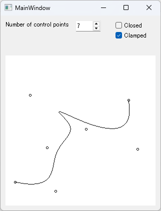
Continuity of B-spline
Curve segments of B-spline considered here are cubic functions of $t$, so the curve segments are twice differentiable and C2 continuous.56
Continuity between curve segments can be determined as C2 continuity by following method:
Let the $i$th and $i+1$th curve segments be:
\begin{array}{l}
\boldsymbol{S}_i(t) =
\begin{bmatrix} t^3 & t^2 & t & 1 \end{bmatrix}
{\boldsymbol{R}}_i {\boldsymbol{P}}_i =
\begin{bmatrix} b_{i_{0,3}}(t) & b_{i_{1,3}}(t) &b_{i_{2,3}}(t) &b_{i_{3,3}}(t) \end{bmatrix}
{\boldsymbol{P}}_i \\
\boldsymbol{S}_{i+1}(t) =
\begin{bmatrix} t^3 & t^2 & t & 1 \end{bmatrix}
{\boldsymbol{R}}_{i+1} {\boldsymbol{P}}_{i+1} =
\begin{bmatrix} b_{{i+1}_{0,3}}(t) & b_{{i+1}_{1,3}}(t) &b_{{i+1}_{2,3}}(t) &b_{{i+1}_{3,3}}(t) \end{bmatrix}
{\boldsymbol{P}}_{i+1}
\end{array}
where
{\boldsymbol{P}}_i =
\begin{bmatrix}
{\boldsymbol{p}}_i \\
{\boldsymbol{p}}_{i+1} \\
{\boldsymbol{p}}_{i+2} \\
{\boldsymbol{p}}_{i+3}
\end{bmatrix}
, \quad
{\boldsymbol{P}}_{i+1} =
\begin{bmatrix}
{\boldsymbol{p}}_{i+1} \\
{\boldsymbol{p}}_{i+2} \\
{\boldsymbol{p}}_{i+3} \\
{\boldsymbol{p}}_{i+4}
\end{bmatrix}
If
\begin{array}{l}
b_{i_{0,3}}(1)=0 \\
b_{i_{1,3}}(1)=b_{{i+1}_{0,3}}(0) \\
b_{i_{2,3}}(1)=b_{{i+1}_{1,3}}(0) \\
b_{i_{3,3}}(1)=b_{{i+1}_{2,3}}(0) \\
b_{{i+1}_{3,3}}(0)=0
\end{array}
then
\boldsymbol{S}_i(1)=\boldsymbol{S}_{i+1}(0)
for any control points, so it can be determined to be C0 continuous.
For open B-spline curves, the coefficient matrix is:
{\boldsymbol{R}}_i={\boldsymbol{R}}_{i+1}=
\begin{bmatrix}
-\frac{1}{6} & \frac{1}{2} & -\frac{1}{2} & \frac{1}{6} \\
\frac{1}{2} & -1 & \frac{1}{2} & 0 \\
-\frac{1}{2} & 0 & \frac{1}{2} & 0 \\
\frac{1}{6} & \frac{2}{3} & \frac{1}{6} & 0
\end{bmatrix}
Substituting this for
\begin{array}{l}
\begin{bmatrix} b_{i_{0,3}}(t) & b_{i_{1,3}}(t) &b_{i_{2,3}}(t) &b_{i_{3,3}}(t) \end{bmatrix} =
\begin{bmatrix} t^3 & t^2 & t & 1 \end{bmatrix}{\boldsymbol{R}}_i
\\
\begin{bmatrix} b_{{i+1}_{0,3}}(t) & b_{{i+1}_{1,3}}(t) &b_{{i+1}_{2,3}}(t) &b_{{i+1}_{3,3}}(t) \end{bmatrix} =
\begin{bmatrix} t^3 & t^2 & t & 1 \end{bmatrix}{\boldsymbol{R}}_{i+1}
\end{array}
we get:
\begin{array}{l}
\begin{bmatrix} b_{i_{0,3}}(1) & b_{i_{1,3}}(1) &b_{i_{2,3}}(1) &b_{i_{3,3}}(1) \end{bmatrix}
=
\frac{1}{6}\begin{bmatrix} 0 & 1 & 4 & 1 \end{bmatrix} \\
\begin{bmatrix} b_{{i+1}_{0,3}}(0) & b_{{i+1}_{1,3}}(0) &b_{{i+1}_{2,3}}(0) &b_{{i+1}_{3,3}}(0) \end{bmatrix}
=
\frac{1}{6}\begin{bmatrix} 1 & 4 & 1 & 0 \end{bmatrix}\end{array}
so C0 continuity can be determined.
The continuity of C1 and C2 can be determined similarly from the first and second derivatives of the basis functions:
\begin{array}{l}
\begin{bmatrix} b'_{i_{0,3}}(1) & b'_{i_{1,3}}(1) &b'_{i_{2,3}}(1) &b'_{i_{3,3}}(1) \end{bmatrix}
=
\frac{1}{2}\begin{bmatrix} 0 & -1 & 0 & 1 \end{bmatrix} \\
\begin{bmatrix} b'_{{i+1}_{0,3}}(0) & b'_{{i+1}_{1,3}}(0) &b'_{{i+1}_{2,3}}(0) &b'_{{i+1}_{3,3}}(0) \end{bmatrix}
=
\frac{1}{2}\begin{bmatrix} -1 & 0 & 1 & 0 \end{bmatrix}\end{array}
so C1 continuity can be determined.
\begin{array}{l}
\begin{bmatrix} b''_{i_{0,3}}(1) & b''_{i_{1,3}}(1) &b''_{i_{2,3}}(1) &b''_{i_{3,3}}(1) \end{bmatrix}
=
\begin{bmatrix} 0 & 1 & -2 & 1 \end{bmatrix} \\
\begin{bmatrix} b''_{{i+1}_{0,3}}(0) & b''_{{i+1}_{1,3}}(0) &b''_{{i+1}_{2,3}}(0) &b''_{{i+1}_{3,3}}(0) \end{bmatrix}
=
\begin{bmatrix} 1 & -2 & 1 & 0 \end{bmatrix}\end{array}
so C2 continuity can be determined.
Clamped B-spline curves have a various coefficient matrix, so a table is used.
C0 continuity can be determined from the following table:
| $m$ | curve segment |
$t$ | $b_{0,3}(0)$ | $b_{1,3}(0)$ | $b_{2,3}(0)$ | $b_{3,3}(0)$ | judge | |
|---|---|---|---|---|---|---|---|---|
| $b_{0,3}(1)$ | $b_{1,3}(1)$ | $b_{2,3}(1)$ | $b_{3,3}(1)$ | |||||
| $5$ | $0$ | $0$ | $1$ | $0$ | $0$ | $0$ | ||
| $1$ | $0$ | $\frac{1}{4}$ | $\frac{1}{2}$ | $\frac{1}{4}$ | $true$ | |||
| $1$ | $0$ | $\frac{1}{4}$ | $\frac{1}{2}$ | $\frac{1}{4}$ | $0$ | |||
| $1$ | $0$ | $0$ | $0$ | $1$ | ||||
| $6$ | $0$ | $0$ | $1$ | $0$ | $0$ | $0$ | ||
| $1$ | $0$ | $\frac{1}{4}$ | $\frac{7}{12}$ | $\frac{1}{6}$ | $true$ | |||
| $1$ | $0$ | $\frac{1}{4}$ | $\frac{7}{12}$ | $\frac{1}{6}$ | $0$ | |||
| $1$ | $0$ | $\frac{1}{6}$ | $\frac{7}{12}$ | $\frac{1}{4}$ | $true$ | |||
| $2$ | $0$ | $\frac{1}{6}$ | $\frac{7}{12}$ | $\frac{1}{4}$ | $0$ | |||
| $1$ | $0$ | $0$ | $0$ | $1$ | ||||
| $\ge 7$ | $0$ | $0$ | $1$ | $0$ | $0$ | $0$ | ||
| $1$ | $0$ | $\frac{1}{4}$ | $\frac{7}{12}$ | $\frac{1}{6}$ | $true$ | |||
| $1$ | $0$ | $\frac{1}{4}$ | $\frac{7}{12}$ | $\frac{1}{6}$ | $0$ | |||
| $1$ | $0$ | $\frac{1}{6}$ | $\frac{2}{3}$ | $\frac{1}{6}$ | $true$ | |||
| $2$ to $m-6$ | $0$ | $\frac{1}{6}$ | $\frac{2}{3}$ | $\frac{1}{6}$ | $0$ | |||
| $1$ | $0$ | $\frac{1}{6}$ | $\frac{2}{3}$ | $\frac{1}{6}$ | $true$ | |||
| $m-5$ | $0$ | $\frac{1}{6}$ | $\frac{2}{3}$ | $\frac{1}{6}$ | $0$ | |||
| $1$ | $0$ | $\frac{1}{6}$ | $\frac{7}{12}$ | $\frac{1}{4}$ | $true$ | |||
| $m-4$ | $0$ | $\frac{1}{6}$ | $\frac{7}{12}$ | $\frac{1}{4}$ | $0$ | |||
| $1$ | $0$ | $0$ | $0$ | $1$ |
C1 continuity can be determined from the following table:
| $m$ | curve segment |
$t$ | $b'_{0,3}(0)$ | $b'_{1,3}(0)$ | $b'_{2,3}(0)$ | $b'_{3,3}(0)$ | judge | |
|---|---|---|---|---|---|---|---|---|
| $b'_{0,3}(1)$ | $b'_{1,3}(1)$ | $b'_{2,3}(1)$ | $b'_{3,3}(1)$ | |||||
| $5$ | $0$ | $0$ | $-3$ | $3$ | $0$ | $0$ | ||
| $1$ | $0$ | $-\frac{3}{4}$ | $0$ | $\frac{3}{4}$ | $true$ | |||
| $1$ | $0$ | $-\frac{3}{4}$ | $0$ | $\frac{3}{4}$ | $0$ | |||
| $1$ | $0$ | $0$ | $-3$ | $3$ | ||||
| $6$ | $0$ | $0$ | $-3$ | $3$ | $0$ | $0$ | ||
| $1$ | $0$ | $-\frac{3}{4}$ | $\frac{1}{4}$ | $\frac{1}{2}$ | $true$ | |||
| $1$ | $0$ | $-\frac{3}{4}$ | $\frac{1}{4}$ | $\frac{1}{2}$ | $0$ | |||
| $1$ | $0$ | $-\frac{1}{2}$ | $-\frac{1}{4}$ | $\frac{3}{4}$ | $true$ | |||
| $2$ | $0$ | $-\frac{1}{2}$ | $-\frac{1}{4}$ | $\frac{3}{4}$ | $0$ | |||
| $1$ | $0$ | $0$ | $-3$ | $3$ | ||||
| $\ge 7$ | $0$ | $0$ | $-3$ | $3$ | $0$ | $0$ | ||
| $1$ | $0$ | $-\frac{3}{4}$ | $\frac{1}{4}$ | $\frac{1}{2}$ | $true$ | |||
| $1$ | $0$ | $-\frac{3}{4}$ | $\frac{1}{4}$ | $\frac{1}{2}$ | $0$ | |||
| $1$ | $0$ | $-\frac{1}{2}$ | $0$ | $\frac{1}{2}$ | $true$ | |||
| $2$ to $m-6$ | $0$ | $-\frac{1}{2}$ | $0$ | $\frac{1}{2}$ | $0$ | |||
| $1$ | $0$ | $-\frac{1}{2}$ | $0$ | $\frac{1}{2}$ | $true$ | |||
| $m-5$ | $0$ | $-\frac{1}{2}$ | $0$ | $\frac{1}{2}$ | $0$ | |||
| $1$ | $0$ | $-\frac{1}{2}$ | $-\frac{1}{4}$ | $\frac{3}{4}$ | $true$ | |||
| $m-4$ | $0$ | $-\frac{1}{2}$ | $-\frac{1}{4}$ | $\frac{3}{4}$ | $0$ | |||
| $1$ | $0$ | $0$ | $-3$ | $3$ |
C2 continuity can be determined from the following table:
| $m$ | curve segment |
$t$ | $b''_{0,3}(0)$ | $b''_{1,3}(0)$ | $b''_{2,3}(0)$ | $b''_{3,3}(0)$ | judge | |
|---|---|---|---|---|---|---|---|---|
| $b''_{0,3}(1)$ | $b''_{1,3}(1)$ | $b''_{2,3}(1)$ | $b''_{3,3}(1)$ | |||||
| $5$ | $0$ | $0$ | $6$ | $-9$ | $3$ | $0$ | ||
| $1$ | $0$ | $\frac{3}{2}$ | $-3$ | $\frac{3}{2}$ | $true$ | |||
| $1$ | $0$ | $\frac{3}{2}$ | $-3$ | $\frac{3}{2}$ | $0$ | |||
| $1$ | $0$ | $3$ | $-9$ | $6$ | ||||
| $6$ | $0$ | $0$ | $6$ | $-9$ | $3$ | $0$ | ||
| $1$ | $0$ | $\frac{3}{2}$ | $-\frac{5}{2}$ | $1$ | $true$ | |||
| $1$ | $0$ | $\frac{3}{2}$ | $-\frac{5}{2}$ | $1$ | $0$ | |||
| $1$ | $0$ | $1$ | $-\frac{5}{2}$ | $\frac{3}{2}$ | $true$ | |||
| $2$ | $0$ | $1$ | $-\frac{5}{2}$ | $\frac{3}{2}$ | $0$ | |||
| $1$ | $0$ | $3$ | $-9$ | $6$ | ||||
| $\ge 7$ | $0$ | $0$ | $6$ | $-9$ | $3$ | $0$ | ||
| $1$ | $0$ | $\frac{3}{2}$ | $-\frac{5}{2}$ | $1$ | $true$ | |||
| $1$ | $0$ | $\frac{3}{2}$ | $-\frac{5}{2}$ | $1$ | $0$ | |||
| $1$ | $0$ | $1$ | $-2$ | $1$ | $true$ | |||
| $2$ to $m-6$ | $0$ | $1$ | $-2$ | $1$ | $0$ | |||
| $1$ | $0$ | $1$ | $-2$ | $1$ | $true$ | |||
| $m-5$ | $0$ | $1$ | $-2$ | $1$ | $0$ | |||
| $1$ | $0$ | $1$ | $-\frac{5}{2}$ | $\frac{3}{2}$ | $true$ | |||
| $m-4$ | $0$ | $1$ | $-\frac{5}{2}$ | $\frac{3}{2}$ | $0$ | |||
| $1$ | $0$ | $3$ | $-9$ | $6$ |
-
B-spline Curves: Definition
https://pages.mtu.edu/~shene/COURSES/cs3621/NOTES/spline/B-spline/bspline-curve.html ↩ -
Carl de Boor
A Practical Guide to Splines, P.132
ISBN 0-387-90356-9 ↩ -
Elaine Cohen, Richard F. Riesenfeld
General Matrix Representations for Bezier and B-spline Curves
Computers in Industry 3 (1982) 9-15
https://www.sciencedirect.com/science/article/abs/pii/0166361582900276 ↩ -
Wikipedia -- Bézier curve
https://en.wikipedia.org/wiki/B%C3%A9zier_curve ↩ -
Gerald Farin
Curves and Surfaces for Computer Aided Geometric Design: A Practical Guide, pp.77-90
ISBN 0-12-249050-9 ↩ -
Wikipedia -- Smoothness
https://en.wikipedia.org/wiki/Smoothness ↩