pixyzでAttentive Neural Processesを実装する

Attentive Neural Processesの実装をpixyzで行った．
準備として，Gaussian Process， Neural Processも簡単に実装した．
(pixyzを使った別の実装記事)

論文について一言で言うと，Attentive Neural Processは，Neural Processがunderfittingである問題をAttentionの枠組みを用いることによって解決したモデルである(詳しい説明は下スライド参照)．

Gaussian Process (GP)

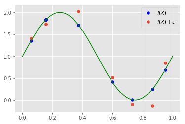
ガウス過程による回帰

訓練データを条件として，新しいデータが与えられたとき，関数fの分布$p(Y^* |X^*, X, Y)$を予測することが目標である．

ここで，X, Yは訓練データ，$X^* $は新しいデータ点， $Y^* = f(X^* )$である
データにはノイズが乗っていることを仮定する

y = f(x) + \epsilon \\
\epsilon \sim N(0, \sigma_y^2) \\
f(x) = \sin (2\pi x) + 1 

%matplotlib inline
import matplotlib.pyplot as plt
import numpy as np
from scipy import linalg as LA
plt.style.use("ggplot")

sigma_y = 0.2

N = 8
np.random.seed(42)
train_X = np.random.uniform(0, 1, N)
train_y = np.sin(2 * np.pi * train_X) + np.random.normal(0, sigma_y, N) + 1
plt.plot(np.linspace(0,1), np.sin(2 * np.pi * np.linspace(0, 1)) + 1, "g")
plt.scatter(train_X, np.sin(2 * np.pi * train_X)+1, c="b", label=r"$f(X)$") # ノイズがのってないデータ
plt.scatter(train_X, train_y, label=r"$f(X) + \epsilon$") # 訓練データ
plt.legend()
plt.show()

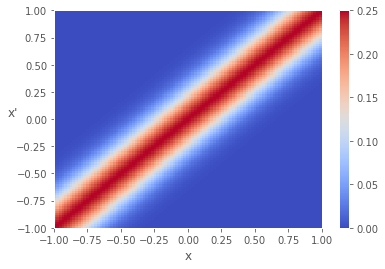
カーネル関数

データの位置が近いと値が大きくなるようなカーネル関数を考える

k(x, x') = \sigma_f^2 \exp (-\frac{1}{2l^2}(x-x')^2) \\
K = k(X^*, X^*)

sigma_f = 0.5 # 垂直の変化のスケールのハイパーパラメタ
l = 0.2 # 水平の変化のスケールのハイパーパラメタ

def k(x, y):
    return sigma_f ** 2 * np.exp(- ((x - y) ** 2) / (2 * l ** 2))

Nx = 100
x = np.linspace(-1, 1, Nx)
X, Y = np.meshgrid(x, x)
K = np.vectorize(k)(X, Y)

plt.pcolor(X, Y, K, cmap=plt.cm.coolwarm)
plt.colorbar()
plt.xlabel("x")
plt.ylabel("x'", rotation=0)
plt.show()

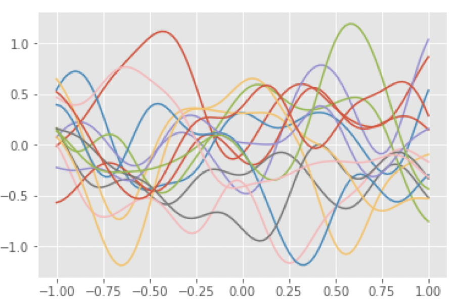
事前分布からのサンプリング

先程定義したカーネル関数を使って，事前分布から関数をサンプリングする

$$
f \sim P(f) = N(f | 0, K)
$$

for i in range(15):
    y = np.random.multivariate_normal(x*0 , K)
    plt.plot(x, y)

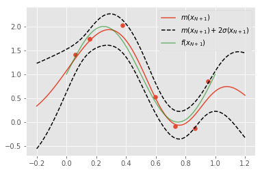
事後分布の表示

導出はPRML6章を参照

y_{N+1} \sim p(y_{N+1} |X, Y, x_{N+1}) = N(y_{N+1}|m(x_{N+1}), \sigma^2(x_{N+1})) \\
m(x_{N+1}) = k(x_{N+1}, X)K_y^{-1}y \\
\sigma^2(x_{N+1}) = k(x_{N+1}, x_{N+1}) - k(x_{N+1}, X)K_y^{-1}k(X, x_{N+1}) 

ただし，$K_y = K + \sigma_y^2 I $である

# ハイパーパラメタ
sigma_f = 0.5
l = 0.2
sigma_y = 0.2

def k(x, y):
    return sigma_f ** 2 * np.exp(- ((x - y) ** 2) / (2 * l ** 2))

def k_(x):
    return np.vectorize(lambda x, y: k(x, y))(train_X, x)

def m(x):
    return K_y_inv.dot(train_y).dot(k_(x))

def sd(x):
    return np.sqrt(k(x, x) - k_(x).dot(K_y_inv).dot(k_(x)))

X, Y = np.meshgrid(train_X, train_X)
K = np.vectorize(k)(X, Y)  #(N, N) ノイズが乗ってないデータ(f(x))の同時分布の共分散
K_y = K + sigma_y ** 2 * np.eye(len(train_X)) #(N, N)  ノイズが乗ったデータ(y)の同時分布の共分散
K_y_inv = LA.inv(K_y)

# 可視化
Nx = 100
x = np.linspace(-0.2, 1.2, Nx)
y_mean = np.vectorize(m)(x)
y_upper = y_mean + np.vectorize(sd)(x) * 2  # 上2シグマ
y_under = y_mean - np.vectorize(sd)(x) * 2 # 下2シグマ

plt.scatter(train_X, train_y)
plt.plot(x, y_mean, label=r"$m(x_{N+1})$")
plt.plot(x, y_upper, "k--", label=r"$m(x_{N+1}) + 2\sigma(x_{N+1})$")
plt.plot(x, y_under, "k--")
plt.plot(np.linspace(0,1), np.sin(2 * np.pi * np.linspace(0, 1)) + 1, "g", alpha=0.5, label=r"$f(x_{N+1})$") # f(x)
plt.legend()
plt.show()

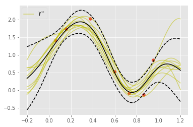
事後分布からのサンプリング

p(Y^*|X^*, X, Y) = N(Y^*|\mu^*, \Sigma^*) \\
\mu^* = K(X^*, X)^TK_y^{-1}y \\
\Sigma^* = K(X^*, X^*) - K(X^*, X)^TK_y^{-1}K(X, X^*)

K_ = np.array([k_(i) for i in x]) # (Nx, N)
X, Y = np.meshgrid(x, x)
K__ = np.vectorize(k)(X, Y) # (Nx, Nx)
mu = K_.dot(K_y_inv).dot(train_y) # (Nx, )
Sigma = K__ - K_.dot(K_y_inv).dot(K_.T) # (Nx, Nx)

# 可視化
plt.scatter(train_X, train_y)
for i in range(10):
    y = np.random.multivariate_normal(mu, Sigma) # 関数のサンプリング
    if i == 0:
        plt.plot(x, y, alpha=0.5, c="y", label=r"$Y^*$")
    else:
        plt.plot(x, y, alpha=0.5, c="y")


plt.plot(x, y_mean, "k")
plt.plot(x, y_upper, "k--")
plt.plot(x, y_under, "k--")
plt.legend()
plt.show()

for i in range(15):
    y = np.random.multivariate_normal(mu, Sigma)
    plt.plot(x, y)

Neural Process (NP)

パラメータ数が多くないので，GPUを使う必要がなかった．
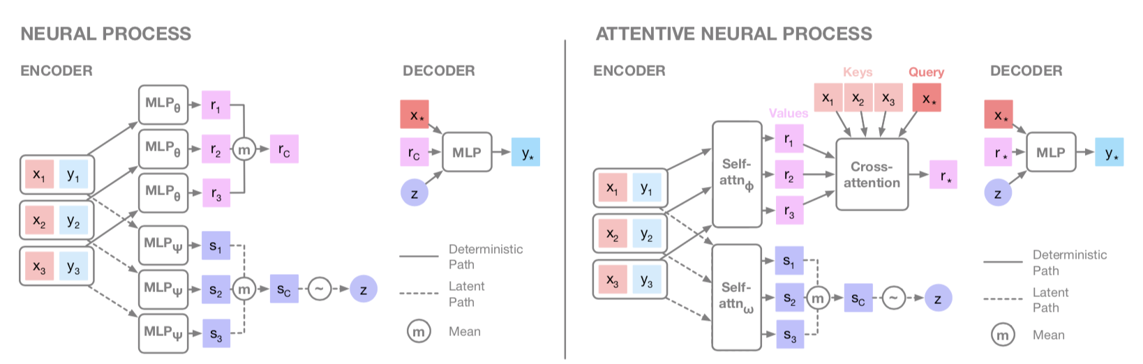
基本的にNPとANPは下の図の通りに実装していく．

import torch
import torch.optim as optim
import torch.nn as nn
from torch.nn import functional as F
from pixyz.distributions import Normal, Deterministic

from sklearn.utils import shuffle

device = torch.device("cuda" if torch.cuda.is_available() else "cpu")
print("device:", device)

# model
class R_encoder(Deterministic):
    def __init__(self, x_dim, y_dim, d_dim, z_dim):
        super(R_encoder, self).__init__(cond_var=["x", "y"], var=["r"])

        self.fc1 = nn.Linear(x_dim+y_dim, d_dim)
        self.fc2 = nn.Linear(d_dim, d_dim)
        self.fc3 = nn.Linear(d_dim, z_dim)

    def forward(self, x, y):
        r = torch.cat([x, y], dim=1)
        r = torch.sigmoid(self.fc1(r))
        r = torch.sigmoid(self.fc2(r))
        r = self.fc3(r)
        return {"r": r}

class S_encoder(Normal):
    def __init__(self, x_dim, y_dim, d_dim, z_dim):
        super(S_encoder, self).__init__(cond_var=["x", "y"], var=["z"])

        self.z_dim = z_dim
        self.fc1 = nn.Linear(x_dim+y_dim, d_dim)
        self.fc2 = nn.Linear(d_dim, d_dim)
        self.fc3 = nn.Linear(d_dim, d_dim)
        self.fc4 = nn.Linear(d_dim, d_dim)
        self.fc5 = nn.Linear(d_dim, z_dim*2)

    def forward(self, x, y):
        z = torch.cat([x, y], dim=1)
        z = torch.sigmoid(self.fc1(z))
        z = torch.sigmoid(self.fc2(z))
        z = torch.sigmoid(self.fc3(z).mean(0))
        z = torch.sigmoid(self.fc4(z))
        z = self.fc5(z)
        z_mu = z[:self.z_dim]
        z_scale = 0.1 + 0.9*F.softplus(z[self.z_dim:])
        return {"loc": z_mu, "scale": z_scale}

class Decoder(Normal):
    def __init__(self, x_dim, y_dim, d_dim, z_dim, init_func=torch.nn.init.normal_):
        super(Decoder, self).__init__(cond_var=["x_", "r", "z"], var=["y_"])
        self.y_dim = y_dim
        self.fc1 = nn.Linear(x_dim+z_dim*2, d_dim)
        self.fc2 = nn.Linear(d_dim, d_dim)
        self.fc3 = nn.Linear(d_dim, d_dim)
        self.fc4 = nn.Linear(d_dim, y_dim*2)

        if init_func is not None:
            init_func(self.fc1.weight)
            init_func(self.fc2.weight)
            init_func(self.fc3.weight)
            init_func(self.fc4.weight)

    def forward(self, x_, r, z):
        y = torch.cat([x_, r, z], dim=1)
        y = torch.sigmoid(self.fc1(y))
        y = torch.sigmoid(self.fc2(y))
        y = torch.sigmoid(self.fc3(y))
        y = self.fc4(y)

        y_mu = y[:, :self.y_dim]
        y_scale = 0.1 + 0.9*F.softplus(y[:, self.y_dim:])
        return {"loc": y_mu, "scale": y_scale}

def context_target_random_split(train_X, train_y):
    N = train_X.shape[0]
    perm = np.random.permutation(np.arange(N))
    train_X, train_y = train_X[perm], train_y[perm]

    N_c = np.random.choice(np.arange(1, N))
    x_c, y_c = train_X[:N_c], train_y[:N_c]
    x_t, y_t = train_X[N_c:], train_y[N_c:]
    return x_c, x_t, y_c, y_t

# パラメータ
z_dim = 3
d_dim = 128
x_dim = 1
y_dim = 1

r_encoder = R_encoder(x_dim, y_dim, d_dim, z_dim).to(device) # (x,y)->r
s_encoder = S_encoder(x_dim, y_dim, d_dim, z_dim).to(device) # (x,y)->z
s_encoder_context = s_encoder.replace_var(x="x_c", y="y_c").to(device)
decoder = Decoder(x_dim, y_dim, d_dim, z_dim).to(device) # (x*, r, z) -> y*
opt = torch.optim.Adam(list(decoder.parameters())+list(r_encoder.parameters())+
                       list(s_encoder.parameters()), 1e-3)

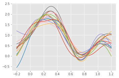
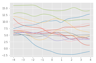
事前分布からのサンプリング

x_grid = torch.from_numpy(np.arange(-4, 4, 0.1).reshape(-1,1).astype(np.float32)).to(device)
for i in range(15):
    untrained_zs = torch.from_numpy(np.random.normal(size=(z_dim)).astype(np.float32)).to(device)
    mu = decoder.sample_mean({"x_": x_grid, "r": untrained_zs.repeat(len(x_grid), 1), "z": untrained_zs.repeat(len(x_grid), 1)})
    plt.plot(x_grid.cpu().data.numpy(), mu.cpu().data.numpy(), linewidth=1)
plt.show()

zの次元にもよるが，表現力の高い関数がサンプルされることがわかる

NPの訓練

ELBOの最大化を行う

\log p(y_{m+1:n}|x_{1:n}, y_{1:m}) \geq E_{q(z|x_{m+1:n},y_{m+1:n})} \left[ \sum_{i=m+1}^n \log p(y_i|z, r_{1:m}, x_i) + \log \frac{q(z|x_{1:m}, y_{1:m})}{q(z|x_{m+1:n}, y_{m+1:n})} \right]

nは訓練データ数，mはcontextの数，n-mはtargetの数．
epochごとに，mはランダムに決め，訓練データはシャッフルする．

# torch tensorに変換
train_X_ = torch.from_numpy(train_X.astype("float32")).to(device)
train_y_ = torch.from_numpy(train_y.astype("float32")).to(device)

# 訓練
for i in range(20000):
    opt.zero_grad()

    # context target split
    x_c, x_t, y_c, y_t = context_target_random_split(train_X_[:, None], train_y_[:, None])
    x_ct = torch.cat([x_c, x_t], dim=0)
    y_ct = torch.cat([y_c, y_t], dim=0)

    # deterministic path
    r_mean = r_encoder(x_c, y_c)["r"].mean(0) # aggregate

    # latent path
    z_sample_target = s_encoder.sample({"x": x_t, "y": y_t})

    # Loss
    nll = - decoder.log_likelihood({"x_": x_t, "r": r_mean.repeat(len(x_t), 1), "z": z_sample_target["z"].repeat(len(x_t), 1), "y_": y_t})
    kl = s_encoder.log_likelihood(z_sample_target) - s_encoder_context.log_likelihood({"x_c": x_c, "y_c": y_c, "z": z_sample_target["z"]})
    loss = nll.mean() + kl.mean()

    loss.backward()
    opt.step()


    # visualize
    if ((i+1)%200)==0:
        Nx = 100
        x = np.linspace(-0.2, 1.2, Nx)
        x_ = torch.from_numpy(x.astype("float32")).to(device)
        r_mean = r_encoder(x_ct, y_ct)["r"].mean(0)
        for j in range(10):
            z = s_encoder.sample({"x": x_ct, "y": y_ct})["z"]
            y_ = decoder.sample_mean({"x_": x_[:, None], "r": r_mean.repeat(len(x_), 1), "z": z.repeat(len(x_), 1)})
            y_ = y_.detach().cpu().numpy()
            if j == 0:
                plt.plot(x, y_, alpha=0.5, c="b",label="NP sample")
            else:
                plt.plot(x, y_, alpha=0.5, c="b")


        plt.scatter(train_X, train_y)
        plt.title("epoch: {}".format(i+1))
        plt.xlim(-0.22, 1.22)
        plt.ylim(-0.55, 2.4)
        plt.plot(x, y_mean, "k", label="GP mean")
        plt.plot(x, y_upper, "k--", label="GP 2sigma")
        plt.plot(x, y_under, "k--")
        plt.legend(loc='upper right')
        plt.savefig("./NP_png/{}".format(i+1))
        plt.show()

ガウス過程の結果とは程遠い結果となった．

Attentive Neural Process (ANP)

NPにCross-Atttention(CA)機構を追加する

• query: x*
• key: x
• value: r

NPとANPの違いは主にこの図でわかる．rを単純に平均をとるのではなく，CAを使う．

Attention部分のより詳細な図

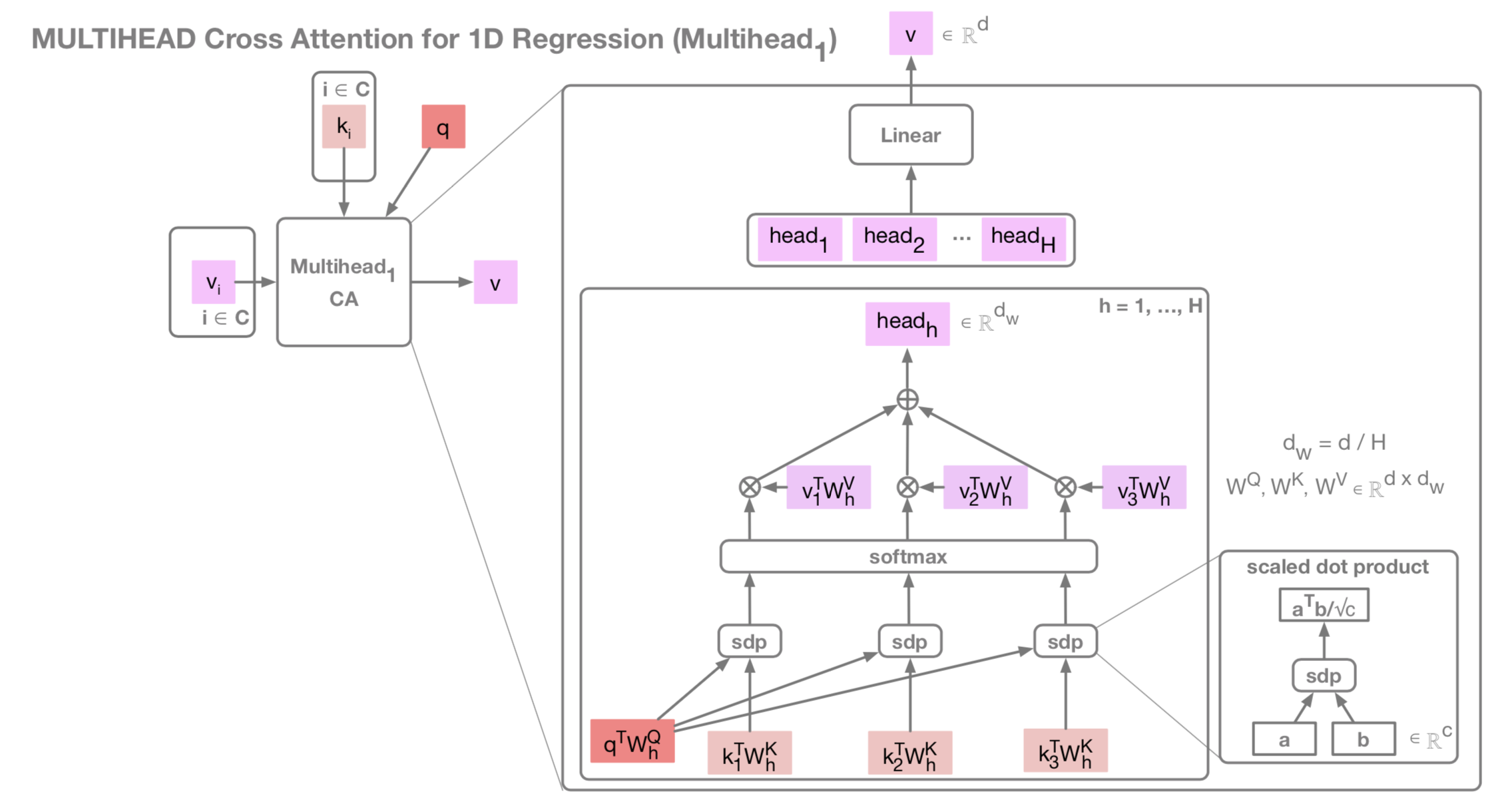
本来はMultihead CAだが，簡単のためSinglehead(=DotProduct) CAで実装している．

# single head model
class CrossAttention(Deterministic):
    def __init__(self, x_dim, d_dim, z_dim):
        super(CrossAttention, self).__init__(cond_var=["x_t", "x_c", "r"], var=["r_"])

        self.fc_q = nn.Linear(x_dim, d_dim)
        self.fc_k = nn.Linear(x_dim, d_dim)
        self.fc_v = nn.Linear(z_dim, d_dim)
        self.fc_h = nn.Linear(x_dim, z_dim)

    def forward(self, x_t, x_c, r):
        q = self.fc_q(x_t)
        k = self.fc_k(x_c)
        v = self.fc_v(r)

        sdp = torch.matmul(q, k.t()) / np.sqrt(k.shape[0]) # scaled dot product
        qk = F.softmax(sdp, dim=1)
        head = torch.matmul(qk, v).sum(1).unsqueeze(1)
        return {"r_": self.fc_h(head)}

z_dim = 2
d_dim = 128
x_dim = 1
y_dim = 1

r_encoder = R_encoder(x_dim, y_dim, d_dim, z_dim).to(device) # (x,y)->r
s_encoder = S_encoder(x_dim, y_dim, d_dim, z_dim).to(device) # (x,y)->z
s_encoder_context = s_encoder.replace_var(x="x_c", y="y_c").to(device)
CA = CrossAttention(x_dim, d_dim, z_dim).to(device) # (x_t, x_c, r)->r_
decoder = Decoder(x_dim, y_dim, d_dim, z_dim).to(device) # (x*, z) -> y*
opt = torch.optim.Adam(list(decoder.parameters())+list(r_encoder.parameters())+
                       list(s_encoder.parameters())+list(CA.parameters()), 1e-3)


# 訓練
for epoch in range(20000):
    opt.zero_grad()

    # context target split
    x_c, x_t, y_c, y_t = context_target_random_split(train_X_[:, None], train_y_[:, None])
    x_ct = torch.cat([x_c, x_t], dim=0)
    y_ct = torch.cat([y_c, y_t], dim=0)

    # deterministic path
    r = r_encoder(x_c, y_c)["r"]
    r = CA(x_t, x_c, r)["r_"]  # ATTENTION

    z_sample_target = s_encoder.sample({"x": x_t, "y": y_t})

    # Loss
    nll = - decoder.log_likelihood({"x_": x_t, "r": r, "z": z_sample_target["z"].repeat(len(x_t), 1), "y_": y_t})
    kl = s_encoder.log_likelihood(z_sample_target) - s_encoder_context.log_likelihood({"x_c": x_c, "y_c": y_c, "z": z_sample_target["z"]})
    loss = nll.mean() + kl.mean()
    loss.backward()
    opt.step()

    # visualize
    if ((epoch+1)%200)==0:
        Nx = 100
        x = np.linspace(-0.2, 1.2, Nx)
        x_ = torch.from_numpy(x.astype("float32")).to(device)
        r = r_encoder(x_ct, y_ct)["r"]
        r = CA(x_[:, None], x_ct, r)["r_"]
        for j in range(10):
            z = s_encoder.sample({"x": x_ct, "y": y_ct})["z"]
            x_ = torch.from_numpy(x.astype("float32")).to(device)
            y_ = decoder.sample_mean({"x_": x_[:, None], "r": r, "z": z.repeat(len(x_), 1)})
            y_ = y_.detach().cpu().numpy()
            if j == 0:
                plt.plot(x, y_, alpha=0.5, c="b",label="ANP sample")
            else:
                plt.plot(x, y_, alpha=0.5, c="b")


        plt.scatter(train_X, train_y)
        plt.title("epoch: {}".format(epoch+1))
        plt.xlim(-0.22, 1.22)
        plt.ylim(-0.55, 2.4)
        plt.plot(x, y_mean, "k", label="GP mean")
        plt.plot(x, y_upper, "k--", label="GP 2sigma")
        plt.plot(x, y_under, "k--")
        plt.legend(loc='upper right')
        plt.savefig("./ANP_png/{}".format(epoch+1))
        plt.show()

最終的に点推定のような結果にしかならない...もし実装が間違っていたら教えてほしいです．

---

実装コード: https://github.com/HironoOkamoto/practice_pixyz/tree/master/NeuralProcess
参考実装: https://chrisorm.github.io/NGP.html
pixyzの公式: https://github.com/masa-su/pixyz