Pytorch で自動運転モデルの学習

目的

こちらの記事 にて Pytorch で自動運転モデルの学習手順が紹介されていたので、自身でその手順を追えるか確かめてみました。その実施内容を以下に示します。

環境・データ

• Google Colabratory
• Pytorch 1.1.0
• csv, 画像データ一式

手順

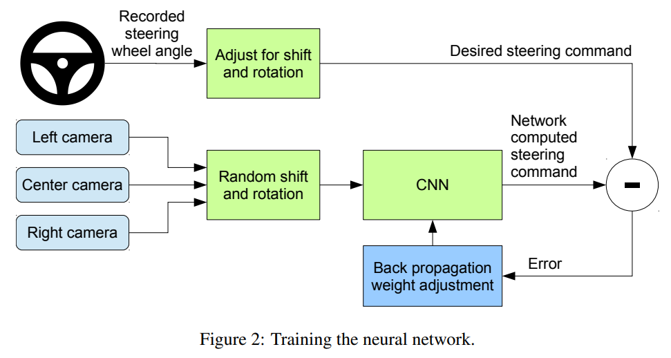
今回実施内容としては こちらの論文 にある通り 運転シミュレータの前面・左・右カメラ画面の画像およびステアリング角を入力として、CNN にて自動運転モデルの学習を行うこと です。

0. 学習データのダウンロード

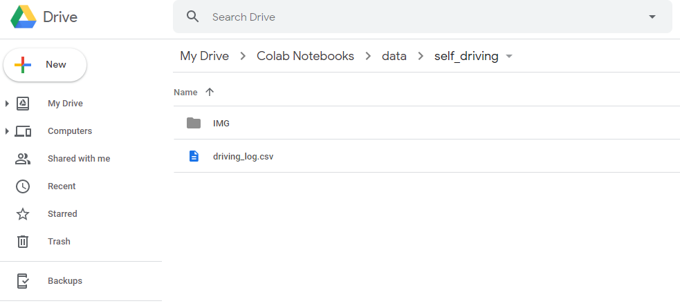
こちら をダウンロードし、zip 展開した data フォルダの中身一式を Google Drive の My Drive > Colab Notebooks > data > self_driving 以下に配置します。

1. Google Colab へログイン

ブラウザから Google Colab にアクセスして、ファイル > Python3 の新しいノートブックを選択し、開きます。

ノートブック画面で ランタイム > ランタイムのタイプを変更 を選択し、ハードウェアアクセラレータをデフォルトの "None" から "GPU" に変更します。

2. ノートブックの編集

ノートブックのコードセルに下記一つずつ順番に入力し、Shift + Enter にて実行していきます（全実行結果はこちら）。

2.1 Google Drive のマウント等を実施します。

# Googleドライブのマウント
from google.colab import drive
drive.mount('/content/drive')

# ライブラリインポート
import torch
import torch.nn as nn
import torch.optim as optim
from torch.utils import data
from torch.utils.data import DataLoader
import torchvision.transforms as transforms
import cv2
import numpy as np
import csv

# Googleドライブのパス設定
import sys
sys.path.append('/content/drive/"My Drive"/"Colab Notebooks"/')
%cd /content/drive/"My Drive"/"Colab Notebooks"/

# GPU 利用可否
print(torch.cuda.is_available())
device = 'cuda' if torch.cuda.is_available() else 'cpu'

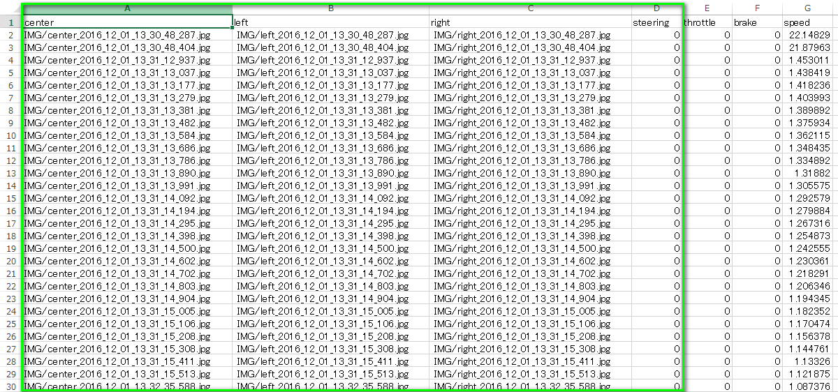
2.2 画像データのパスおよびステアリング角度が記載された csvファイルを読み込みます。

読み込む csv データの中身は下記です。ここでは緑枠のデータのみ利用します。

# Step1: Read from the log file
samples = []
with open('data/self_driving/driving_log.csv') as csvfile:
    reader = csv.reader(csvfile)
    next(reader, None)
    for line in reader:
        samples.append(line)

2.3 学習に使うデータと検証に使うデータを分けます。

ここでは 8割のデータを学習用とし、残りを検証用としています。

# Step2: Divide the data into training set and validation set
train_len = int(0.8*len(samples))
valid_len = len(samples) - train_len
train_samples, validation_samples = data.random_split(samples, lengths=[train_len, valid_len])

2.4 データ引数およびデータセットのクラスを定義します。

# Step3a: Define the augmentation, transformation processes, parameters and dataset for dataloader
def augment(imgName, angle):
  name = 'data/self_driving/IMG/' + imgName.split('/')[-1]
  current_image = cv2.imread(name)
  current_image = current_image[65:-25, :, :]
  if np.random.rand() < 0.5:
    current_image = cv2.flip(current_image, 1)
    angle = angle * -1.0  
  return current_image, angle

class Dataset(data.Dataset):

    def __init__(self, samples, transform=None):
        self.samples = samples
        self.transform = transform

    def __getitem__(self, index):
        batch_samples = self.samples[index]
        steering_angle = float(batch_samples[3])
        center_img, steering_angle_center = augment(batch_samples[0], steering_angle)
        left_img, steering_angle_left = augment(batch_samples[1], steering_angle + 0.4)
        right_img, steering_angle_right = augment(batch_samples[2], steering_angle - 0.4)
        center_img = self.transform(center_img)
        left_img = self.transform(left_img)
        right_img = self.transform(right_img)
        return (center_img, steering_angle_center), (left_img, steering_angle_left), (right_img, steering_angle_right)

    def __len__(self):
        return len(self.samples)

2.5 データセットし、バッチサイズおよびコア数を指定してデータローダを作ります。

ここで、バッチサイズは32とし、コア数（"num_workers" は 4）としました。

# Step3b: Creating generator using the dataloader to parallasize the process
transformations = transforms.Compose([transforms.Lambda(lambda x: (x / 255.0) - 0.5)])

params = {'batch_size': 32,
          'shuffle': True,
          'num_workers': 4}

training_set = Dataset(train_samples, transformations)
training_generator = DataLoader(training_set, **params)

validation_set = Dataset(validation_samples, transformations)
validation_generator = DataLoader(validation_set, **params)

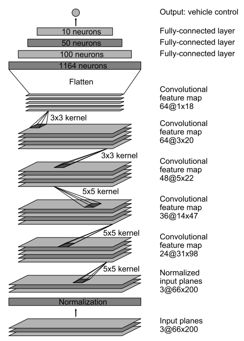
2.6 ネットワークの定義

CNN ネットワーク構成を 論文 のFigure 4 のものと同様に定義したものは下記です。

# Step4: Define the network
class NetworkDense(nn.Module):

    def __init__(self):
        super(NetworkDense, self).__init__()
        self.conv_layers = nn.Sequential(
            nn.Conv2d(3, 24, 5, stride=2),
            nn.ELU(),
            nn.Conv2d(24, 36, 5, stride=2),
            nn.ELU(),
            nn.Conv2d(36, 48, 5, stride=2),
            nn.ELU(),
            nn.Conv2d(48, 64, 3),
            nn.ELU(),
            nn.Conv2d(64, 64, 3),
            nn.Dropout(0.25)
        )
        self.linear_layers = nn.Sequential(
            nn.Linear(in_features=64 * 2 * 33, out_features=100),
            nn.ELU(),
            nn.Linear(in_features=100, out_features=50),
            nn.ELU(),
            nn.Linear(in_features=50, out_features=10),
            nn.Linear(in_features=10, out_features=1)
        )

    def forward(self, input):  
        input = input.view(input.size(0), 3, 70, 320)
        output = self.conv_layers(input)
        output = output.view(output.size(0), -1)
        output = self.linear_layers(output)
        return output

ただし、こちらでは計算時間の便宜上、下記のように 論文 に示されているネットワークより計算量の少ないネットワークを定義し、計算実行自体はそちらで行います（※動作確認が目的のため）。

class NetworkLight(nn.Module):

    def __init__(self):
        super(NetworkLight, self).__init__()
        self.conv_layers = nn.Sequential(
            nn.Conv2d(3, 24, 3, stride=2),
            nn.ELU(),
            nn.Conv2d(24, 48, 3, stride=2),
            nn.MaxPool2d(4, stride=4),
            nn.Dropout(p=0.25)
        )
        self.linear_layers = nn.Sequential(
            nn.Linear(in_features=48*4*19, out_features=50),
            nn.ELU(),
            nn.Linear(in_features=50, out_features=10),
            nn.Linear(in_features=10, out_features=1)
        )


    def forward(self, input):
        input = input.view(input.size(0), 3, 70, 320)
        output = self.conv_layers(input)
        output = output.view(output.size(0), -1)
        output = self.linear_layers(output)
        return output

2.7 最適化アルゴリズムおよび損失関数を定義します。

最適化アルゴリズムは Adam, 損失関数は平均二乗誤差関数を使っています。

# Step5: Define optimizer
model = NetworkLight().to(device)
optimizer = optim.Adam(model.parameters(), lr=0.001)

criterion = nn.MSELoss()

2.8 学習実行します。

25エポックの学習をさせてます。100バッチごとの損失および1エポック実施後の損失の平均値を出力させています。

def toDevice(datas, device):

  imgs, angles = datas
  return imgs.float().to(device), angles.float().to(device)

max_epochs = 25

train_loss_list = []

for epoch in range(max_epochs):

    # Training
    train_loss = 0
    model.train()
    for local_batch, (centers, lefts, rights) in enumerate(training_generator):
        centers, lefts, rights = toDevice(centers, device), toDevice(lefts, device), toDevice(rights, device)

        optimizer.zero_grad()
        datas = [centers, lefts, rights]        
        for i, data in enumerate(datas):
            imgs, angles = data
            outputs = model(imgs)
            loss = criterion(outputs, angles.unsqueeze(1))
            loss.backward()
            optimizer.step()
            train_loss += loss.data.item()
        if local_batch % 100 == 0:
            print('Loss: %.3f ' % (train_loss/(local_batch+1)))

    avg_train_loss = train_loss / len(training_generator.dataset)

    print ('Epoch [{}/{}], Loss: {loss:.4f}' 
                   .format(epoch+1, max_epochs, local_batch+1, loss=avg_train_loss))
    train_loss_list.append(avg_train_loss)

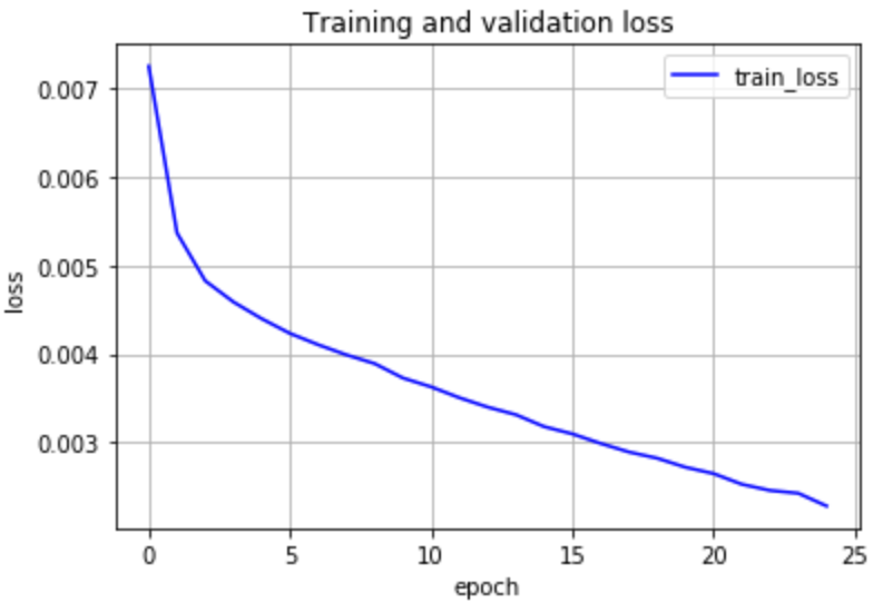
2.9 エポックが進むにつれて損失が減少していく様子の図示

横軸をエポック、縦軸を損失としてグラフを出力させます。学習が進むにつれて損失が減っている様子が確認できます。

結果：

import matplotlib.pyplot as plt
%matplotlib inline

plt.figure()
plt.plot(range(max_epochs), train_loss_list, color='blue', linestyle='-', label='train_loss')
plt.legend()
plt.xlabel('epoch')
plt.ylabel('loss')
plt.title('Training and validation loss')
plt.grid()

参考

• Deep Learning for Self-Driving Cars
• End to End Learning for Self-Driving Cars